But there are still times when you need to know more about an opamp you are considering.
The picture below shows an early opamp tester used to flesh out some concepts. It's not clear if it will become a product or not as it is rather specialized. The tester is USB powered and allows you to learn a lot about an opamp under conditions that might be important to you but might not be present on the data sheet.
There are a lot of relays on the board, and the generalized schematic appears as below:
The various connections options above might not make sense, but depending on the switch configuration, you can get the following configurations:
Some of these configurations will make perfect sense. But others might not. The thread HERE on the forum surfaces two interesting papers that will explain much of the above.
The first is Samuel Groner's extensive work (HERE) on characterizing opamps. Groner looks at distortion contributions based on input, output and loading.
The second paper (HERE) is by former Burr Brown engineer Jerald G Graeme. In that paper Graeme explains way to modify the signal gain and distortion/noise gain of the opamp separately. For example, you can see in Configuration 5A in the plot above a circuit with signal gain of -10 and a distortion/noise gain of 10. This corresponds to Figure 3 on page 6 of the Graeme PDF. Note in Graeme's circuit the addition of a resistor between the - and + terminals of the opamp (R3). This resistor allows you set a different gain for the error term of the opamp. Referring back to the Configuration of 5B above, the error term gain is 4.99K/(499||49.9) = 110.
It's a similar exercise for the the non-inverting case (configurations 6A and 6B). Those are shown here:
The DUT opamp used in this case is an LM358 (even though the plots say LM386--that is incorrect).
Here we can see configuration 6A (no distortion multiplier). Note the signal gain is 0 dB as expected. And we can see the THD is about -107.
Next, we switch to Configuration 6B and run the test again:
Currently there are 13 configurations shown above. These include configurations for measuring noise and CMRR as well as distortion for other gains (inverting and non-inverting). There is also the ability to apply 4 different loads to the opamp (infinity,2K, 600, 470 ohms). For example, below is the LM358 with no load (left) and 470 ohm load (right):
In the above plots, we can see a change in amplitude based on the load, which means we can calculate the output impedance of the opamp in closed loop configurations.
We can also look at the gain-bandwidth product of an opamp using something like the QA403 with 100 kHz of bandwidth. A really fast opamp that has a GWB of 30 MHz will have its bandwidth reduced as gain is increased. So, a 30 MHz opamp operating with a gain of 1000X will have 30 kHz of bandwidth. The 1000X gain corresponds to Configuration 1.
On the LM358, that plot appears below. Here we can see a frequency response sweep shows the 3dB rolloff occurs at 1003 Hz at 60 dB of gain. Backing out the gain, this means the GBW would 1.003 MHz. The spec sheet says the GBP of this LM358 variant is 700 kHz.
The hardware can also test PSRR of the positive and negative rails separately, and can measure input offsets. The hardware also has adjustable rails ranging from +/- 0.1V up to the full +/- 15V. And the rails can sense current, allowing Iq to be measured as well as opamp efficiency.
Over the coming months, work will be done to automate more of the tests. It should be a fun side project.
Feel free to discuss this post HERE.
If you liked the post you just read, please consider signing up for our mailing list at the bottom of the page.
]]>
But what if you need to test something that isn't supported by Tractor out of the box? If your testing needs are complex, then writing your own software is one option. This can allow you to control every aspect of testing down to the smallest detail. But another option is to add the test to Tractor.
You don't need to be a software whiz to do this. If you can recognize patterns and do a tiny bit of programming, you can probably create your own test.
Suppose, for example, you wanted to measure the noise in a power amplifier between 30 and 40 kHz to look for a problem that occurs on some units due to an engineering issue. Normally, Tractor works at a fixed 48 kHz sampling rate. You'd need at least an 80 kHz sampling rate to make the RMS measurement from 30 to 40 kHz.
Let's see how we could solve this.
1) Install Visual Studio 2022 from Microsoft. The community edition is free and will work fine. It's located here. You'll be building the Tractor app which is written in C#, so make sure to install the C# options.
2) Download the Tractor source from Github. It's located here. On this page, you'll see a green button called "Code", and if you click on that, you'll see the option to download a ZIP file of the project. Click the "Download ZIP" option.
3) Unzip the zip into the directory of your choice.
4) Start Visual Studio 2022, and do a File-Open Project and select the QA Tractor.SLN file in the unzipped directory.
5) From the main menu in Visual Studio, pick Build->Build Solution. You will probably get two errors about the "mark of the web." This might sound scary, but this is Visual Studio telling you that the files came from the web and to be careful. You will need to mark the files as safe. Using the file explorer, navigate to each file in the directory you unzipped. Right click on the file, select "properties" and tick the "unblock"
6) Close Visual Studio, and re-start it. And then re-load the QA Tractor.sln file. The project should now build. Press the green "START" button at the top of the Visual Studio tool bar and the application should run.
7) OK, so let's add a method to permit us to switch the QA40x to a higher sample rate. On the right side of Visual Studio, look for the Solution Explorer. Drill down as shown below until you locate the file QA40x.cs. Double click on that to open the source to that file.
8) When the file opens, around line 53 add the following lines:
public void SetSampleRate(int sampleRate)
{
PutSync(string.Format($"/Settings/SampleRate/{sampleRate}"));
}
When added it, should appear as follows:
9) Run the application again, and verify it starts.
10) Next, go back into the solution explorer and locate the file RmsLevelA01.cs.
11) Right click on this and select Copy. And then, select the parent directory called "GainLevel". Right click on that and select paste. You should now have a copy of that file as shown:
12) Right click on the file we just copied and re-name it to MyRmsLevelA01.cs
13) Now, if you try to run, you'll have several errors. That is because you've duplicated a class name. So, open the MyRmsLevelA01.cs file and change the class name on line 11 to MyRmsLevelA01:
14) Next, there is still an error. We need to change the name of the constructor as shown:
15) Next, start Tractor again, and add a test. Set the Test Category to LevelGain, and you'll now see the test we added as an option.
16) If you add the test to your test plan, it will work exactly as it did before, which isn't very helpful. But now, let's add code to set the analyzer to a higher sample rate. To do this, navigate to around line 43 of the MyRmsLevelA01.cs file and add the following line:
((QA40x)Tm.TestClass).SetSampleRate(96000);
The above line will call the code we added in the QA40x.cs file at the top of this post. Note that the line following this line is using an IAudioAnalyzer cast, while this line we added is using a QA40x cast. That means this test is specific to the QA40x products and wouldn't work on the QA401.
The result should appear as follows:
Let's talk about what is happening above. The DoTest() method is called when it's time for this test to run. In line 40, we put the analyzer into a default state. The next line sets some common parameters like FFT length, muting, etc.
The line 43 we added then sets the sample rate to 96ksps, using the method (function) we added earlier.
17) Next, move up to lines 23 and 26 in the file, and set the MaxValue for the RMS measurement Start and Stop to be 48000 as shown. Without this change, we'd still be at the higher sample rate but we couldn't enter frequencies higher than 20 kHz.
18) Now run the app, and you should be able to add the test and set the RMS measurement window from 30k to 40k.
19) Now run the test, and you'll should see the sample rate get set to 96k on the analyzer, and the RMS measurement you requested will be made in the band you specified.
And because this is your custom test, you can change everything you need about the test to function as needed. You could even add code to control other instruments, such as power supplies.
]]>The front-panel of the QA440 is shown below:
The front-panel of the QA440 has two DB25 connectors. The connectors expose 15 group of conductors as shown below:
Relays inside the box allow you to connect Group 1 or Group 2 to Group 3, and Group 4 or Group 5 to Group 6, etc. The UI for the QA440 is exposed as follows:
From the above, it should be clear how you can select the various routings. From the primitives, some very sophisticated routings can be had. For example, you can create 5 2:1 muxes, or 3 2:1 muxes, and a 3:1 mux, or a 4:1 mux and a 3:1 mux. There are lots of possibilities. The full list is shown at the wiki located HERE.
For 5.1 testing, the aim is to provide 6 channels of measurement.
The test board is show below. The size is 610 mm wide and 145 mm tall.
For the 5.1 test board, there were a few goals:
0) Demonstration only (this isn't a product for sale)
1) Power handling to 500W/channel
2) Built-in attenuation
3) Up to 6 channels
4) Direct connection to the QA440
The power handling was achieved using ARCOL loads. These loads are discussed in more detail in the post HERE. In short, they are very low-cost, non-inductive, and very rugged. The loads are mounted in a piece of laser-cut 1/8" aluminum to help with thermal dissipation.
Attenuation is achieved using a simple resistive divider, and are discussed in more detail HERE.
Up to six channels can be supported. In the picture above, just 5 loads are shown. Above each load is a red + black screw terminal for connecting to the amp.
The DB25's shown in the upper right of the test board are for connection to the QA440.
The laser cut aluminum piece is shown below. The various cutouts are relief for the various through-hole connectors. Mounting holes for the loads are shown. Those were tapped upon receipt.
The PCB connection detail for the loads is shown below. To connect, the load leads are trimmed and soldered to a pad on the PCB:
The routing for the PCB was selected to ensure all traces flowed cleanly without any jumpers being needed and keeping most all routing to the top layer:
A 5.1 amplifier has 6 independent amplifiers. Above, we used a 6:1 mux to test each amplifier sequentially, while ensuring all amps were under load. The signal paths were balanced, meaning each measurement had a + and - signal.
If your amp wasn't balanced, you might be able to do a stereo 6:1, though each channel wouldn't be independent.
Another approach would be a 3:1 mux, and measure as stereo pairs (front left and front right, back left and back right, and then measure center channel and sub together). The wiki linked above shows the various configuration options. This configuration would offer independent control of each 3:1 mux (and you'd get a spare 2:1 mux).
A 7.1 amplifier has 8 channels to measure, or 4 stereo pairs. Since an 8:1 mux cannot be realized with the QA440, if the amp is unbalanced you could do 4:1. If the amp is balanced, however, there aren't enough relays to make the measurement. In this case, the operator could be prompted to manually swap some cabling. Or potentially another QA440 could be used.
Be aware: the connection choices can be bewildering at times. Draw a picture (as shown above) where you clearly identify the pins for each relay and the connection diagram and double and triple check your work. Connector assignments are the most error-prone phase of design work usually.
For certain measurements, the standard two channel option isn't convenient. But a relay board and some custom hardware can make it easy to automate more difficult configurations. In the example above, a custom board was made to permit a generic 6:1 loaded measurement.
Feel free to discuss this post HERE.
If you liked the post you just read, please consider signing up for our mailing list at the bottom of the page.
]]>Here we are a year later, facing a problem that might seem similar but is actually much more severe: the current silicon shortage is an unprecedented event. And it continues to get worse. In the last blog post I outlined a metric (% of TI DCDC converters that are in stock at Digikey) and began tracking that in June of this year. Since that time, we've seen Digikey stock levels continue to fall with no end in site. The graph below shows the deterioration, and the message is simple: Digikey has less than 40% of TI's DCDC converter parts in stock. Normally, in good times, this would be north of 85%. And for the remaining 15% that were out of stock at Digikey, you could get them at another distributor. But parts are out everywhere.
We use several of the SN6505B in most every product we make. Below is Octopart's summary on the availability: Nobody has any parts. Some brokers in Asia will list availability, but they either don't have parts (eg they aren't being truthful in their reporting to Octopart) OR they are expecting to receive $40 for $1 part.
But this can't last forever, right? How bad can this be? Most distributors never dreamed you'd need visibility into the supply pipeline, and so they don't let you see precisely when they are expecting parts. However, Mouser does give you a snapshot of when they have parts scheduled to arrive.
Here's their take below on when the SN6505B will be arriving--a year from now. Yes, lead time for large orders placed directly from TI today is 81 weeks. Orders placed today will be filled in a year, assuming they are under Mouser's inventory levels.
All of the above is for a simple transformer driver--a simple part used to generate the isolated voltages used in the QA402. The part is unique to TI, but other vendors make something similar though it requires a board re-design to use.
If we go TI's website and use their tools to look at step-down DCDC regulators, we can see they have a huge portfolio of 1332 parts. But when you filter by products for which 10K or more are in stock, just 336 are available. That is, they only have sizable numbers of just 25% of their portfolio.
Now, all of these problems can usually be worked around. You first find a part that is in-stock that does a similar job, buy those parts NOW, and then re-design the board. And then do a few board iterations to get everything just right. But when you need to do that for 15 parts on the board, the tasks is suddenly on-par with doing an entire re-design. And if we're going to do a board re-design, then we're going to re-do a lot more than a few problem parts.
And so, work has been underway for some time on a QA403. The QA403 was supposed to live alongside the QA402, but given the landscape it looks like the QA403 will make it to market before parts for the QA402 arrive. And in other cases, we have parts in the inventory (like the SN6505 mentioned above) but would rather use those parts on a higher-performing analyzer such as the QA403 rather than the QA402.
The QA403 will be our next audio analyzer. Externally, the QA403 will appear just like the QA402. Internally, the QA403 moves to the ES9822PRO for the ADC, and the ES9038Q2M for the DAC. Internal signal-paths move to OPA1612 for noise, and the gain switching structure has been improved.
Benefits include:
* Improved performance (THD, THD+N, noise)
* Reduced power consumption
* 384K sample rate possibility (still TBD)
There is a lot of re-use between the QA403 and QA402. The QA403 will also have the option to be non-isolated. The isolation solution used on the QA402 and QA403 is a major issue, with part lead times rivaling those of the SN6505B outlined above. To work around that, there will be a placement option to build a non-isolated version of the analyzer should the shortage persist. If a person wanted to, it would be easy to convert a non-isolated analyzer to an isolated analyzer: Just remove the 0 ohm jumpers and place the SOIC isolation parts.
The software used for the QA402 will have the QA403 support added, and the QA402 and QA403 will use the same software (the QA40x application). Applications you have written to run on the QA402 will run the QA403, usually with no or very minor changes.
Shipping on the QA403 should begin in February 2022. For those that like seeing the internals, below is a near-final board, but there will be probably be two more releases before production. The cost will be similar to the QA402.
The last 18 months have been about as brutal as could be imagined from a supply perspective. And there's really no end in sight. Daily it appears to be getting worse, not better. But, when the supply issues finally do lessen, it will likely happen fairly quickly because so much additional capacity is being built today. And then we'll be staring down a glut of parts. Such is life.
From a schedule standpoint, it looks like the QA451 will be back in stock next month or January 2022, and the QA460 will be back in January or February as the QA461, with improved current sense monitoring.
So, stay tuned. We'll get through this, but it's going to take some time.
Feel free to discuss this post HERE.
If you liked the post you just read, please consider signing up for our mailing list at the bottom of the page.
]]>The graph below is the mid-September update. Since July we've seen Digikey stock degrade further, by another 8% or so. However, note there's a slight uptick with inventory over the last 6-8 weeks or so.
Good news for now on this metric that may or may not matter in the end.
The graph below shows Digikey's in-stock level for TI DCDC converters. Normally, TI carries about 2800 TI DCDC parts. These are the "normally stocking" checkbox on the webpage. Of the normally stocked parts, currently about 54% are in stock (46% out of stock).
Now, I'm sure TI or Digikey would say "Now, this graph doesn't tell the entire story" and they would be correct. But as long as Digikey is showing daily declines on stock levels, it's probably safe to say we haven't hit bottom. Buckle up.
###
The coming months are going to be difficult in terms of product availability as the semiconductor shortages continue. Normally, when it's time to build a more of a product, the process starts 3-4 weeks before the product is actually needed. Printed circuit boards are ordered from China, and take about 2 weeks to arrive. An order is placed with Digikey or Mouser, and parts arrive in a few days. And then both are taken to the assembly house, where the boards are are assembled in 5-10 days. The process is largely automatic: You decide how many you want, you push a button in automated ordering scripts that generate the bill of materials, and it all just works.
But for the last few months, it's not generally been possible to order everything from a single supplier. It has required purchasing parts from a few different suppliers as not everyone has everything in stock. But in the last month, it's gone to another level of disfunction.
The QA460 uses a part called the TPS62135 to generate a 10.5V rail from a 12V input. If you look on Octopart, there are zero parts anyplace in the system:
And if you look at lead times on Mouser, you can see parts aren't expected until this time next year.
And it's not just a matter of re-designing the board to use another DCDC converter. The situation is equally dire for just about any DCDC converter right now.
The upshot is that until things improve, we're going to have some large inventory gaps in our product portfolio that will manifest in the coming weeks, and they won't be fixable until the shortage starts to resolve. A magnetics supplier told me last week they they will be mostly caught up in late summer. The situation with passive discretes (resistors, capacitors, etc) is mostly fine. But the unique silicon situation is bad right now.
Thanks, Matt
]]>The December 2020 issue overview is HERE.
]]>The solution in this case is to use a known stimulus saved as a WAV file. You can then load this WAV file onto the MP3 player or a USB drive, and play it out of whatever device you'd like to test.
Let's say you were interesting in learning the frequency response of a PC DAC that you were evaluating. You could use PC Mirror mode on the QA401 and step through a series of tones, measuring the amplitude of the tones. Since the PC controls the DAC, and the QA401 software is running on the PC, that would be a straightforward task. But it would be time consuming. Let's take a look at how to do it quickly with a single chirp.
The first task is to compose the chirp. The sample rate of the DAC will be locked at 48 kHz--it's that roll off around 20 kHz we're particularly interested in. So, we'll want the QA401 in 192 kSps mode to ensure the DAC response isn't tempered by the analyzer response. And we'll use a 64K sized FFT. This will complete in well under a second.
Net, we need to consider the level. Let's start with a chirp at -10 dBFS.
Let's start by the putting the QA401 software into a known state: From the file menu, select "Reset Startup Defaults"
Next, change the sample rate (Settings->Options->General) to 192Ksps.
Then, select a 64K FFT size using the FFT control in the ACQ SETTINGS control group.
Switch to DBFS mode using the DBFS button in the AXIS SETTINGS control group. This allows us to specify the amplitude in dBFS, which is appropriate for a DAC.
Next, control+click on the FREQ RESPONSE button in the MEASUREMENTS control group. This will open the FR Settings dialog. Note the amplitude units is in dbFS. Set that to -10 dBFS.
We've now set everything needed to ensure we're in the mode we wanted:
Now, go to the File->Export menu and select Export Chirp. Accept the default file name. The file will be exported to your MyDocs\QuantAsylum\QA401 folder.
The name of the file is
Chirp_Bd32f_Fs192_Le64k_Pb2k_Am-10.0dBFS.wav
Breaking this down, this is a chirp, with a bit depth of 32-bit, expressed as a float (+/-1.0 max), at a sample rate of 192K, with a length of 64K samples, with a pre-buffer of 2K, and at an amplitude of -10 dBFS.
It is very important your settings on the analyzer match the chirp!
We can now play that chirp using whatever WAV file player you prefer. Loading the WAV in Audacity shows the following (you could load the WAV file on your phone, car, too if that is your DUT).
In the plot above, you can roughly two regions. The first region is 10 mS of a 1 kHz sine, following by a sweep starting a low frequencies and rising to very high frequencies. The purpose of the 1 kHz sine in the beggining is to allow the QA401 to trigger. The captured 10 mS of sine will be thrown away, and the analysis will be done on the remaining sweep.
With the WAV loaded and ready to play, you need to tell the analyzer software to get ready to capture. An additional button has been added to the Run/Stop control group:
Pressing the "Open Loop Acq" button bring up a dialog. This dialog will show the left channel streaming data in real time. The capturing will start when the threshold (-35 dBFS in the plot below) is exceeded. Make your you are in the +6 dBV input range if appropriate. Otherwise, you will need a much stronger signal to trigger the acquisition.
Before capturing the signal, make sure you are in the Freq Response mode by pressing the Freq Response button in the MEASUREMENTS control group.
Now, play the WAV file you exported above on your DUT. If the captured signal exceeds the threshold, the resulting spectrum will be displayed. Note the flat passband, and the sharp rolloff after 20 kHz. Since we're in 192k sample rate on the analyzer, and the DAC is locked to 48k, we can be sure this rolloff is due to the DAC and whatever transcoding Windows/Audacity is doing.
Next, open the graphic EQ in Audacity and notch out 1 kHz:
"Preview" the notch while capturing on the QA401 again. Here we see the 1kHz notch appears in the spectrum:
The chirps above about about 0.25 seconds in duration, making the characterization very fast.
Moving the WAV to an Android phone and playing back with Foobar2000 yields a similar response:
Open Loop testing can be very useful for looking at the frequency response of a DUT that doesn't have an analog input readily accessible. The release should post in the next few days.
]]>In late October, a massive 82 hour fire destroyed AKM's ability to deliver their flagship ADC and DAC products to customers, and this included the AK4490 DAC and AK5397 ADC used in the QA401.
This has put enormous pressure on countless companies (including QuantAsylum) that relied on AKM parts. And frankly, given AKM's size, it's surprising they didn't have an alternate fab that was geographically diverse to help insulate them from a severe earthquake (or fire). But alas, here we are.
A follow-on to the QA401--the QA402--has been in the works for a long time and is mostly complete, but the AKM fire has prompted a pivot to new converters. The ADC in the QA402 has been replaced with an PCM4220 from TI and the DAC has been replaced with the PCM1794A.
The purpose of this post is to share some of the details and early measurements on the QA402. And if you've been wanting to buy a QA401, this post will hopefully give you some indication that what is coming is worth waiting for.
The QA402 offers a lot of improvements over the QA401 (all are subject to change, of course). Let's look at a few below.
Lots of input relays. The QA401 had a single stage attenuator of 20 dB, with a max input of +26 dBV (the two input ranges were +6 and +26 dBV max). The QA402 offers two additional relays, ensuring the ADC can be fed at its optimal point over a much larger dynamic range. This manifests on the UI as with the following gain range options as shown below: 7 steps 6 dB apart with the max input being + 36 dBV (the max input on the QA401 was +26 dBV).
All CMOS opamps. The QA401 used a very low-noise bipolar front-end (OPA1612). When your source impedance was below 1K, the performance could not be beat. But at higher source impedances, the noise increased quickly--that is the nature of bipolar. But since the QA401's introduction in 2015, the OPA2156 and its audio cousin the OPA1656 arrived, and they have reset everyone's opinion of CMOS and low noise. This new breed of CMOS opamp is simply phenomenal from a noise and distortion standpoint (though still not as good as bipolar on noise when source impedance is below 1k). And it means there's no longer a painful noise penalty for those times when your source impedance rises above 1k.
Lots of output relays. The QA401 didn't have any output relays. The QA402 has two, offering 0, 10, 20 or 30 dB of output attenuation. The max output of the QA402 is 8Vrms = +18 dBV (single ended) and 16Vrms = +24 dBV (differential). With some higher power amps, the +6 dBV drive of the QA401 was insufficient to let the amp hit max power. The QA402 won't have any problem driving those amps.
USB Powered. The QA401 and QA402 are both USB powered. The current demands on the QA402 are steep--about 5V at 800 mA. But it's no problem for a USB hub to provide. But this means you will most certainly need a powered hub to run the QA402 (or a USB Y-cable if you really want to use your laptop without a hub). Luckily, hubs are cheap and since all our instruments are USB powered (except the QA460), you'll probably want a hub anyway.
Wider Internal Rails. The QA401 uses +/-6V internally for the audio input and output voltage rails. On the QA402, that increases to +/-13V.
Advanced Power Reporting. Because the power demands increased, you will need some advanced diagnostics to ensure your QA402 is running right. The QA402 has the ability to report the USB voltage inside the QA402 as well as the total current AND the current spent on the split rails generation. In the picture below, you can see the QA402 is reporting the USB voltage is at 4.8V, the USB current is 801 mA total, and the current feeding the rail generation DCDC converter is 566 mA (meaning the non-rails current is 801 - 566). These will turn red when a problem is present. For example, a skinny USB cable will have too much voltage drop and you'll see the USB voltage reported as low. Or, if you are driving into a low-impedance load with a high output level, the ISO current will increase (and can hopefully detect and protect the QA402's output stage as accidental shorts at +18 dBV output will be a problem). In short, the pieces are in place to ensure you have the tools to manage the power on the QA402 and verify the QA402 is functioning as designed.
Improved Noise Floor: The QA401 delivered a noise-floor around -115 dBV (20 kHz, no weighting). The QA402 should achieve slightly better. And it's always easy to use an external low-noise amp for those times you need to measure even lower. For example, the QA471's low-noise 30 dB amp let the QA401 measure noise floors down to about -125 dBV (20 kHz, no weighting).
Connectors. The front panel of the QA402 has L/R input XLR (female) and L/R output XLR (male), and also a pair of BNC for single-ended outputs. There's also a digital connector with I2S signals present, so that you can drive some of the newer digital class D power amp ICs directly. That isn't working yet but the path to make it work seems clear.
A picture of the current hardware (REVH PCB) with TI silicon is shown below:
And the performance? Well, the board above with the TI converters has been in-house for 24 hours, and the ADC (driven by the QA480 at +6 dBV) appears as follows.
In single-ended loopback, at -25 dBV out, you can see the DAC + ADC together. The -25 dBV level shows the benefit of the DAC attenuator (0, 10, 20 or 30 dB atten).
In the plot below, you can see ADC sweeps (made with the QA480) showing two different input ranges: +6 dBV max, and +0 dBV max. This gives you an idea of how all the different gain ranges combine. When your input level is around -20 dBV, you'd want to be in the 0 dBV input range. And when your input level is around -14 dBV, you'd want to be in the +6 dBV range. At each point, you keep the distortion optimized, allowing you to deliver very solid distortion numbers across a huge dynamic range. Something a sound card can never do, even when using a state of the art ADC and DAC. And yes, a simple autoranging button will be provided that will allow you optimize for THD or THD+N.
The measurements above don't have all the normal QA401 markers because the software is being re-written. The REST engine from the QA401H was pulled in, which offered a good excuse for a lot of cleanup. This will give a super-clean SW interface for external measurements via REST, making it simple to measure THD from a Python or even Matlab, for example. And if you want headless, then you can "disappear" the GUI and run headless, just as you do with the QA401H today.
And the other reason for the re-write? Here's some very early testing of the QA402 hardware on Ubuntu. Yes, cross platform is coming.
As mentioned in the beginning, this is a very early look at the QA402. The product isn't without risk, but this is all normal at this stage of development. For example, the DAC output levels might be a concern (too large) and have to be dialed back. The I2S might have be abandoned and saved for a second product. The power consumption might end up being too steep. The drive levels might be weak at higher output levels (that is, only high-Z loads can be driven at high output levels). The TI ADC has noise bump at 192Ksps that might be more objectionable than anticipated. THD is where we want, but THD+N isn't quite yet there yet.
In short, right now the expectation is shipping in March 2021 on the new 2.0 cross-platform software (the QA401 will move to that software too and will pick up the cross platform benefits). And the price of the QA402 will be very close to the QA401.
In a perfect world, I think the QA402 with AKM converters would have slightly better performance, but the number of relays on the QA402 means the QA402 performance will be quite a bit better across a larger range than the QA401. Could some more esoteric converters have been used? For sure. But longevity and supply reliability are very important. And TI are very good in those areas.
And finally....Remember, the goal with the QA401 (and QA402) isn't the best performance in the world. That space is well covered if you have the funds. Instead, the goal is to create something that is as trusty as your DVM for audio (meaning no calibration needed) and that has enough performance and margin to reliably measure 99% of the audio products out there today. I think the QA402 will continue to serve that segment very well.
Feel free to discuss this post HERE.
If you liked the post you just read, please consider signing up for our mailing list at the bottom of the page.
]]>Dante (Digital Audio Network Through Ethernet) is a way to move many--up to 1024 uncompressed channels of audio--over a single ethernet cable with incredible reliability and redundancy. Latency is extremely low (sub millisecond), and each endpoint maintains its own clock, meaning the latency at each endpoint can be tailored. This is important in large live sound settings where physical distances can wreak havoc with time alignment.
The larger picture for Dante is that you have lots of audio sources (transmitters) and sinks (receivers). Each of these is connected to the network, and a piece of software on your PC known as a controller allows you to send any transmitter to any receiver or even multiple receivers. So, for live audio, you take all your mics and instruments, plug each into a mostly standard ethernet router and you can then specify in the controller where those packets should all go. For example, they could all go to a front-of-house mixer, and some might go to both the FOH and monitor mixer. The mixed signals could then be sent to speakers over the same ethernet.
And increasingly, we're seeing the input and output of devices speak Dante. So, there is a role here for testing over Dante.
We'll do this using the QA401 and the following pieces:
Dante AVIO Digital Output Adapter This is basically an ethernet to DAC box. This box is plugged into a PoE hub. Price is about $120. In the Dante world, these allow you to connect legacy equipment to the network. For example, if you had a powered speaker with an analog input, you'd use this output adapter to make it Dante-ready. There are ethernet to ADC boxes too, as well as speakers with an ethernet ports (Dante) on the back, amplifiers with Dante inputs. It's a very strong ecosystem with a well thought out silicon portfolio for making existing devices (such as microphones) Dante-ready.
5 Port Gibabit PoE Switch This is a simple ethernet switch with 4 powered ports. These ports follow 802.3af, meaning 48V is provided on the ethernet port, and that is used to power the Output Adaptor above. Nothing too special is needed, and off the shelf stuff will work fine for most setups.
Dante Virtual Soundcard This is what makes Dante work out of the box with the QA401. This software makes the Dante devices appear as a standard sound card. And since the QA401 will use your primary sound card as the "mirror" device, this piece of software can be used to test any Dante receiver. This costs about $30 from Audinate.
Dante Controller This software runs on your PC and lets you configure how all the various receivers and transmitters will talk to each other. This software is free from Audinate.
The setup described below is working via "mirroring". This is a mode on the QA401 where the tone you specify for Gen1 (frequency and amplitude) is "mirrored" out the primary soundcard in the system. You can test Dante receivers using this approach, but you can't test Dante transmitters.
To set things up, we first plug the Avio output adapter into the PoE switch. And then that is plugged into the test PC ethernet port.
Next, install the Dante virtual soundcard and set it up for WDM audio:
Next, in the controller, specify you want Channel 1 on the PC to connect to the Receiver you plugged in above. With WDM, you will get 16 channels of audio.
Then go into your Sound Settings in Windows and find the Dante Virtual Soundcard and set channel 1-2 to be the default audio device. This is how the QA401 knows what soundcard to use:
And at this point, you have set up the Dante side of things. Next, re-start the QA401 and go into Settings->Options->Other and enable Mirroring
With the output of the Dante receiver connected to the input of the QA401, we can switch into dBFS mode and set the generator to -1 dBFS and Enable Gen1:
And then, you should see a tone on the display. This is the tone being generated by the Dante receiver (this is a fully differential measurement--that is, the Pin2 of the XLR goes to the L+ input, and Pin3 of the XLR goes to the L- input).
Note in the plot above we've switched back to dBV, but we're still generating at -1 dBFS from the Dante receiver. And with -1 dBFS input, we see we get about 0.7 dBV out, or about 1Vrms.
Now, we have an option from the Dante controller to adjust some settings on the receiver. One option is to move from the default +4 dBu to +18 dBu (12 dB higher). Let's do it:
That adjustment requires the attenuator to be engaged on the QA401. After doing that, we're met with the following. Note the peak is now 14.16 dBV.
Measuring Dante audio receivers should be pretty straightforward using the QA401 software. Dante is very easy to setup. And by making it your default sound card, you can be making basic measurements just as you would a DAC.
Happy experimenting!
PS. This post can be discussed on the forum at the link HERE.
If you liked the post you just read, please consider signing up for our mailing list at the bottom of the page.
]]>One drawback of the QA450 was the fact that when the loads were disconnected, the output was muted. That changed on the QA451, and the measurement path was decoupled from the load path. This means that on the QA451 you can make measurements of an unloaded amplifier. But it also means you can use an external load in place of the integrated 4 and 8 ohm loads.
The QA451's internal loads are designed for fast burst testing, and with an appropriately sized FFT you can quickly make measurements up to 200W into 8 ohms very quickly (4 ohms will give you roughly twice that, but see the manual for the caveats) . But there are times, especially during development, where it's useful to have much larger resistors sitting in a bucket of water to allow extended testing at very high power levels. With the decoupled inputs of the QA451, this is easy to do. A QA451 user (thanks MP!) shared some external load resistors that I'd not seen before: ARCOL chassis mount. These are thick film, non-inductive resistors with the load element encapsulated inside an aluminum extrusion. Three of the LPR100 series stacked together are about the size of a deck of playing cards. They come in wide range of values, including 4, 6 and 8 ohms. The LPR50 can handle 50 watts, and the LPR100 can handle 100W with a maximum temperature rating of 250C. They can handle 5X the rated load for 5 seconds. And--the best part--a 100W resistor (500W peak) is about $6 in small quantities.
With that, the path to extended testing at 1 kW or even 2 kW is suddenly very clear!
OK, so with these loads, why use the QA451 at all for extended duration testing of Class D? Primarily it's the filter. Take a look below at the hash on the output of a Behringer NX1000. The first plot shows a few full cycles (this is 200W into 4 ohms):
In the plot above, we can see it's roughly 20 volts peak. This is one leg of the output and it's being driven differentially. This is about 40 volts peak across the speaker, which is 28.3 Vrms, which means 200W (the QA401 is reporting 206W). Note the tips of the sine are showing a lot of fuzz--that is the the carrier (aka the switching frequency) of the Class D amp. Let's zoom in and take a closer look at this hash/fuzz. Below you can see a zoom near a zero crossing. What you are seeing here is a zoom of the hash. The class D frequency is about 300 kHz, and the digital hash is about 2.5Vpp (5Vpp differential). That's a lot of hash to ask the audio analyzer to handle by itself.
The QA451's 6th order filter was previously discussed HERE. Given the 300 kHz carrier frequency of the NX1000, we'd expect to see roughly 60 dB of attenuation of the switching frequency based on the plot at the link above. That would take the 5 Vpp and knock it down to around 10 mVpp. And it also converts the signal to a single ended signal.
Outside of the power handling, the QA451 has a maximum input capability that is largely set by the internal +/- 15.5V rails. Remember the QA451 has a 12 dB attenuator on the speaker signal path (the link above has the schematic). And the opamps used are rail to rail input and output. So, we might expect the max swing to about around +/-15.2V or so. With the 12 dB attenuator considered, this means a max input of +/- 60.8V = 43 Vrms = 32.7 dBV, which is 230W into 8 ohms, 462W into 4 ohms, and 925W into 2 ohms.
Let's take a look at the block diagram of the QA451, this time with an external load connected (NOTE: Do NOT engage the internal loads when using an external load! Check the front-panel LEDs of the QA451 to ensure your internal loads are NOT active)
To verify the 15.2V figure we estimated above, let's compare the output of the amplifier with the output of the QA451 at the onset of clipping. In the plot below you can see the amp output (top trace) and the QA451 output (lower trace, with flattened tips). Clearly, you can see that the QA451 has started clipping before the amp has started clipping. The peak to peak is show as 32V = 16Vp, but that's a bit optimistic and the 15.2V or so used above is the more conservative figure.
The spectrum for the above appears as follows: This is about 484W.
So, with the QA451 clipping we know that to hit the 1000W watt mark, we're going to need 6 dB of external attenuation in addition to the 12 dB of attenuation supplied by the QA451.
What we ultimately end up with is a configuration that appears below. Note that the QA451 inputs tap off the lower half the resistors, providing 6 dB of attenuation before the signal hits the QA451. Combined with the QA451's front-end, this gives us 18 dB of attenuation total. This will take the QA451's max handling (due to input swing limitations) from 32.7 dBV to 38.7 dBV = 86.1Vrms. Into 4 ohms, that is 1.8 kW. And it aligns nicely with the 2 kW limitation (5 seconds) offered by the 4 LPC100 resistors.
And a picture of the setup as connected to the Berhinger NX1000 amp:
And with the above, we can run a THD plot on the NX1000 with the following parameters (this is for 64K FFT, and note we've specified the input gain as -18 dB, which is 12 for the QA451 and 6 for the resistor array. We've also specified that the plugin will manage the attenuator, which means the plugin will engage the attenuator as needed to maximize THD or THD+N. The early abort is enabled, which says effectively to 'stop testing if the output power is greater than 10W AND if the THD has degraded beyond -20 dB').
The resulting plot is below with the NX1000 at max volume:
And the THD+N plot appears as follows:
The QA451 is well suited for fast testing on the manufacturing line. But there are times in development where you need to soak up lots more power and for extended intervals. For that, you can use your preferred external load and still get the benefits the QA451 offers: a 6th order filter to knock down Class D switching energy and a clean differential to single ended conversion. With a little bit of wiring, you should have a setup that can test 4 ohms to nearly 2 kW. This same recipe can be readily tweaked to allow 4 kW at 2 ohms, or 1 kW at 8 ohms.
PS. This post can be discussed on the forum at the link HERE.
If you liked the post you just read, please consider signing up for our mailing list at the bottom of the page.
]]>The two DB25 connectors can be configured to provide 7 modes of switching operation, summarized below:
From the table above, you can see Mode 1 provides 5 stereo pairs of muxing, with a single mux pair appearing as follows:
Mode 7 allows you present the switch array as a single 6:1 mux. And of course, there are a lot of options in between. Since the switching mechanism is a relay, it's bi-directional and can be used as a 2:1 mux or 1 of 2 selector.
The various relays are presented on the front panel as follows:
In the picture above, you can see the standard DB25 pin numbers (inside the circles), the various group numbers (1..16, but not only group 1..15 are wired) and the color coding on the DB25 pins. Looking at a single DB25 we have the following:
In the diagram above you can see how the Hot/Cold signals are presented in each group.
All of the relays are under USB control. This allows Tractor to control the relays as part of your test flow. So, if you wanted to test a 5.1 amplifier (6 channels), you'd be able to provide 6 external loads to the amp, and then use the relay box to tap off of each load in sequence, and present those signals to the QA401. And then, under Tractor, you'd select channel 1, test THD, select channel 2, test THD, etc. This would allow you to test all channels under load.
During the factory test of the QA401, there are three configurations tested: All inputs grounded (to check noise), L- and R- ground and L+ and R+ IN to L+ and R- OUT(to check single ended performance), and all inputs driven (to check differential performance). To date, the configuration switching has been done by the operator switching BNC cables and shorting blocks (per on-screen instructions presented by Tractor). A connector board was made (shown below) that connects to the QA440 to automate this IO switching.
In the PCB layout above, note the 4 connectors on the left (each is a "stacked BNC" connector) are spaced to match in the 8 front-panel connectors on the QA401. On the right, is the DB25 connector. This breakout board above is connected to the QA440 using a low-cost "balanced snake" (link HERE at Amazon). While you could make the snake yourself (and there are plenty of how-to articles), the aim to to enable a standard pinout to permit low-cost long-runs of shielded cables to ensure a trouble-free installation in the harsh settings that factories often present.
The board shown above is the pushed onto the BNC connectors of the QA401, and the entire switching process is automated. No more manual cable switching or routing! Of course, you'd make your own PCB to facilitate breaking out the DB25 connector to whatever connector you might need.
Send a mail to the Support alias if you are looking for a relay box to try in your factory setup. First beta units should be ready in a 3-4 weeks.
Thanks, Matt
PS.
PS. This post can be discussed on the forum at the link HERE.
If you liked the post you just read, please consider signing up for our mailing list at the bottom of the page.
]]>In short, the QA490 makes it easy to compare IEMs. But the QA490 cannot answer definitively what the headphone sensitivity is at, say, 10 kHz. That's because the standard for doing so is somewhat arbitrary, and tightly tied to various manufacturer's solutions. We'll discuss that in more detail below.
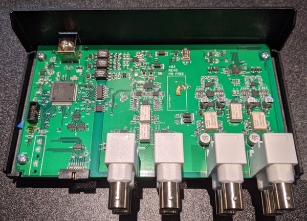
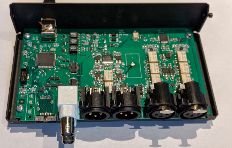
The front panel of the QA490 is shown below.
The LINK LED indicates if the QA490 is connected to the PC and processing commands over USB.
The HI GAIN LED indicates if the QA490 is in high-gain mode. Normally, the QA490 offers a gain of 0 dB, which is suitable for driving most lower-impedance headphones. For headphones with an impedance greater than 100 ohms or so, the high-gain mode will give an extra 12 dB of gain on the input signal. This ensures you can easily drive even 600 ohm headphones to the 25 or 30 mW level with input levels from the driving equipment that are around 1-2 dBV or so. Since the QA401 maximum output is around +6 dBV, this makes it easy to measure high-impedance IEMs and higher power levels. Currently, most high-impedance IEMs are coming in around 150 ohms or so--not quite as high as the over-the-ear headhones. But the drive challenges are still there.
The Z LED indicates the QA490 is in impedance measurement mode. That will be covered in more detail below.
To the right of the LEDs are the ear cups and 1/4" TRS output. The ear cups are where the IEMs are inserted.
To the right of the ear cups are the inputs. These are signals from the QA401. And to the right of the inputs are the outputs. These BNC connectors go back to the QA401.
The block diagram for the QA490 is shown below.
There are two paths to consider. The upper half of the drawing shows the path of the audio input, flowing through the headphone power amp (OPA1622), and finally to the 1/4" front-panel 1/4" TRS. Notice the OPA1622 amps have switchable gain (0 or 12 dB, provided via a relay) and are followed by current sensors. The current sensors are needed to measure the impedance. During normal operation, the current sense resistor is bypassed, ensuring you get the full drive capability (>+/- 100 mA) of the OPA1622. When in current sense mode, a 0.5 ohm series R is switched into the path, along with a difference amp with a gain of 20. Combined, this gives an effective output Z of 10 ohms, but only burdens the output with the 0.5 ohm sense resistor. This ensures that while measuring the impedance you are still able drive low impedance IEMs without much drop across the current sense resistor.
In the normal mode of operation (Z LED is off), the output from the front panel is the signal from the MEMS mics. There are two MEMS mics (one for left, one for right), each positioned on the PCB at the base of the front ear cups.
The structure of each ear cup appears as follows (cross section shown, with the IEMs being inserted from the right side of the drawing). Note that the IEM is inserted into a 10.5mm diameter cup. An acoustic channel, roughly 12mm in length and 3 mm in diameter, delivers the sound from the IEM down to the MEMS mic. The MEMS mic is shown in red atop the green PCB, with the mic port centered in the channel.
If you are familiar with the evolution of acoustic couplers, then you'll quickly realize this looks nothing like the IEC '318, IEC '711 or any of the other standards that have emerged to model human hearing. All of these couplers have different goals in terms of what they are simulating. And even among each coupler standard there are huge variations that can be seen if you change a dimension just a bit. And since human ear canals can vary in length by 30-50%, it should be pretty clear this isn't an exact science. What might give a flat response on one human doesn't on another.
A good drawing of the ear with dimensions and some crude statistics is located HERE. A typical IEM will be inserted about 10 mm into the ear canal. Thus, the coupler above, with a 12 mm path length mimics a 22mm canal length.
Now, it might seem like it would make a lot of sense to try and exactly replicate the ear dimensions. But then you'd need to consider the material, the fact that there's a drum at one end, and on and on. In the end, while it could be done, it could only be done for a single person. But what that person hears is nothing like what the next person hears--similar, yes, but not the same. So there's a compromise that must always be made.
As stated at the top of this post, the aim isn't a perfect absolute measurement. Instead, the aim is a very repeatable relative measurement across a certain frequency range so that two hopefully identical IEMs can be compared. And if they appear nearly identical in the measurements, then we can assume the IEM that was questionable (aka the DUT) was manufactured correctly.
Below we'll look at a few different areas:
Sensitivity: This is the SPL output from the IEM at a specific frequency (usually 1 kHz). This can be readily estimated.
Frequency Response: This is the biggest wildcard, and the primary reason the QA490 is for looking at relative (instead of absolute) performance.
Impedance: Because impedance doesn't require an acoustic measurement, there is no uncertainty with this measurement.
IEM Isolation and Noise Cancellation: This is a measure of how much ambient noise is reduced for the listener. It can occur passively (isolation) or actively (cancellation).
The MEMS mics used on the QA490 are TDK/InvenSense ICS40619 top-port mics. The key specs on the mic are below, but keep in the mind the mic is used in a single-ended fashion, so the sensitivity is - 6 dB less than what is shown. The mics also have excellent matching: the +/-1 spec is worst case. The acoustic overload point is 132 dBSPL (A-weighted), and the dynamic range is 105 dB below the AOP (27 dBSPL)--this is the equivalent input noise. If you've had notions that MEMS mics were inferior, they are not. Their consistency and huge dynamic range are leading and also the way forward. Massive investment from the industry is flowing into MEMS as these mics are enabling much of the innovation you see in the smart assistant space. Moving forward, expect to see further refinement around noise, flatness and bandwidth coming.
From the spec above, we know that if we hit the mic with a 1 kHz 94 dBSPL tone in a free field that the mic will output -44 dBV on each output, 180 degrees out of phase (remember the QA490 uses a single output internally) and these combine to the rated -38 dBV figure above. The way the mic is being used in the QA490 isn't free space--it's in a confined tube, has no porting, and thus it's probably more like a pressure field. The upshot of the enclosed environment (eg. IEM coupled via tube to microphone) probably doesn't match the free-space measurements.
Let's make some first sensitivity measurements with a Shure SE215-CL headphones. These are modestly priced $99 headphones with a clear spec on sensitivity: 107 dB SPL/mW @ 1 kHz.
So, if we hit the headphones with precisely 1 mW, then that should result in a 107 dB SPL. The coupler path will exhibit some loss (or gain), and the mic will see the post-loss level and generate an output signal based on that. What we need to determine is what the loss the coupler looks like.
The process depends on us knowing the precise impedance of the headphones. The measured value is just over 16 ohms. The procedure for making that measurement is shown below.
Next, in the QA401 application we can specify the load impedance via the dBV context menu:
In the QA490 application, we want to adjust the routing so that we can monitor the voltage across the headphone's impedance. We do this by selecting the Left Z mode. In this mode, the routing inside the QA490 will be modified so that the left channel output is the voltage across the left channel (measured directly across the IEM), and the right channel will be the current flowing into the left channel of the IEM. When you are in this mode, the Z LED will be illuminated on the front panel to alert you this isn't the normal mode of operation.
We can then adjust the generator level until we see precisely 1 mW being delivered to the headphones (note below how clean the signal is--there's no distortion from the OPA1622. This is another clue that the signal you are looking at is the electrical signal and not the mic signal).
Now, we move back to the default routing (without changing any levels on the QA401):
The QA401 display is now showing the mic output level, and we can see that figure is 63.5 mVrms = -23.9 dBV. So, we know that when we drove a 1 mW/1 kHz tone into the headphones, the headphones emitted a tone that was 107 dBSPL (based on Shure specification), and the mic responded with an output that was -23.9 dBV, which is 20.1 dB above the -44 dBV @ 94 dBSPL sensitivity. This suggests the level seen by the mic is 94 + 20.1 = 114.1 dB.
Now, at this point, we have a discrepancy to rationalize, and that value is about 114.1 - 107 dB = 7.1 dB--that is, it's 7.1 dB higher than we'd expect. Now, the Shure IEMs could be putting out more volume than expected (eg their sensitivity is higher than the spec). Modern manufacturing should probably have that down to +/- 2 dB or better. And the mic is spec'd to within +/- 1 dB. But, we also have a gain or loss from the coupler that isn't yet understood.
So, for now, let's note that it appears that 107 dBSPL generates -23.9 dBV. Which means that 94 dBSPL of IEM output would generate -36.9 dBV.
FiiO FH1s are well regarded IEMs with a rated sensitivity of 106 dBSPL/mW. The measured impedance of these headphones is 26.7 ohms. With 1 mW into the IEMs, the output is -23.7 dBV.
With the FiiO , it appears that 106 dBSPL generates -23.7 dBV. That is very close to the -23.9 dBV value measured above. This means 94 dBSPL would deliver -35.7 dBSPL.
So, the Shure are -36.9 dBV @ 94 dBSPL, and the FiiO are -35.7 dBV @ 94 dBSPL
If we split the difference, that gives a sensitivity of -36.3 dBV @ 94 dBSPL. Let's call it -36 dBV @ 94 dBSPL. This probably isn't broadly applicable to all IEMs. You will need to estimate for your IEMs them based on established acoustic measurement in your own lab.
Once we have a rough sensitivity established, we can make further readings in absolute dBSPL. If we specify an offset of -(94 - -36) = -130 dB, then we can read dBSPL directly from the display (the peak is at 106.3 dB SPL--if you use the dBR setting, you can change the scale to read dBSPL instead of dBV)
We can also run a stepped chirp response to see where the IEMs start to go into compression. In the test below, we're stepping from -30 dBV output to -4 dBV output, 2 dB per step. What we're looking for in the output plot is where the output no longer increases 2 dB. This will be shown by lines that begin to collapse upon each other.
And in the plot below, we can see around 125 dBSPL and at 2 kHz the output started going into compression:
In the previous section, we used some measurements of some well specified IEMs to derive an approximate sensitivity for the QA490. We can do this at 1 kHz, because everything is well defined at 1 kHz.
Let's take a look now at repeatability of measurements. To do this, we're going to run a frequency response plot on 5 sets of "Adorer EM10 headphones", all new.
But before running the five different sets, let's take a look at the frequency response of the same EM10 IEM measured 6 times without re-fixturing between runs. As expected the repeatability is very good above 100 Hz. We can see some difference between left and right, however. This demonstrates a lower bound on frequency response measurements to keep in mind.
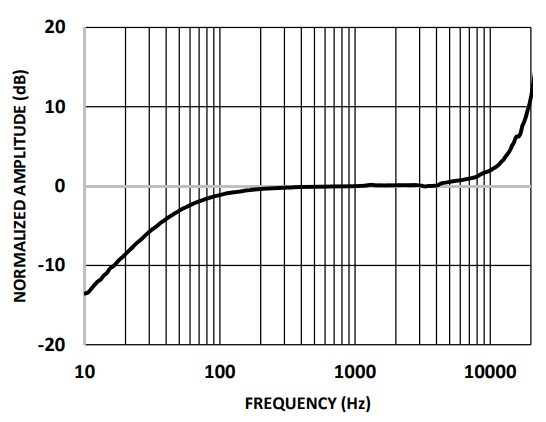
Now, at this stage, it's pretty clear the frequency response isn't flat. Why is that? Let's start by looking the frequency response of the ICS40619 MEMS mic. This is pretty typical for all smaller MEMS mics: At the low-end range there is a roll-off related to the internal volume of the MEMS package. In the high frequency range, there is a resonate peak. In bottom ported mics this resonate peak is generally higher due to the smaller resonances associated with the mechanical structure.
Now, the good news is that the MEMs response is very consistent. But the shape of the MEMS response limits the un-corrected response of the mic to roughly 300 Hz to 8 kHz or so if your aim is uncorrected flatness..Later experiments will look at flattening the response curve through software (and this would also aim to correct resonances that are dependent on the mechanical coupler structure).
Getting back to the measured frequency response and using the same settings as above, let's make one measurement as fixtured, an then reverse the left and to see what changes. In the plot below, note that the variation is related to the IEMs and not the QA490 around mid-band. If the variation was related to the QA490, then you'd expect to see the reds (right channel) bunching together and the blues (left channel) bunching together. And in fact, you do see that happening up around 10 kHz.
Finally, let's take a look at 10 runs of the same IEM, just re-fixtured. That is, make a measurement, remove the IEMs from the earcups, replace the IEMs into the earcups, and then measure again. The goal here is to tease out how sensitive the measurements are to operator placement variation. There's a lot of variation at the low end, and we can see the right channel exhibits a lot of variation around 9 kHz. Let's zoom in a bit more:
Overall, the spread looks very tight from 500 Hz to 8 kHz or so. From this data, we could generate a mask to use as a pass/fail.
Now let's run 5 different sets of EM10 headphones. Here we start to see the manufacturing variations. Above, when the same headphone was run 10 times, note the spread at 1 kHz was around +/- 0.5 dB. In other words, no matter how you fixtured the headphone, the result was nearly the same at 1 kHz.
Zooming in on the above at 1 kHz, we can see more on the spread. The hottest sensitivity was about -39 dBV and the coolest was about -42 dBV. Adding some +/-4 sigma bars take the spread from -36 to -43.5, or about 7.5 dB, or +/- 3.75 dB. That's a barn door, and 4 sigma is a pretty weak quality gate. In short, we'd expect that out of 100 headphones, there's be large, audible difference between the units. No surprise, these are very low-cost headphones.
The unique mechanical structure of the QA490 combined with the frequency response of the QA490's MEMS mics make it very hard to use the QA490 as a device for developing headphones. Instead, as noted above, it should be seen as a device for confirming two headphones match in terms of performance around a few key areas: Sensitivity, frequency response and impedance.
To measure impedance, the HEAD Impedance plug-in can be used:
The options for this plug-in appear as follows. There's not much value in driving the IEMs too hard or too soft. If you drive too hard they may distort, and if you drive too softly the SNR of the measurement will result in a noisy measurement. Keep in mind that most headphones will be used around 80 to 100 dBSPL, so pick a drive value that falls at the higher end of that range. This will help minimize the impact of nearby sounds on the measurement quality.
The impedance plot of the Shure SE215 is shown below. These are 17 ohm headsets according to Shure.
A plot of 5 EM10's is shown below. These are rated as "16 ohms at 1 kHz".
Noise isolation is the amount of noise a set of IEMs will block for the listener. This comes from simply plugging the ear canal. Noise isolation can be learned by playing a white or pink noise source on speakers, and looking at the difference in spectrum. Because these measurements are relative, the QA490 can help reveal the regions where isolation is working well.
In the plot below, you'll see two traces. The green trace is the ambient pickup of the pink noise source. The yellow plot is the with the SE215 inserted (and unpowered). You can see around 1 kHz there's about 15-20 dB of reduction, and around 4-5 kHz there's 30-40 dB of reduction. Shure indicates these IEM blocks "up to 37 dB" of external sound (no information is provided on the frequency), which is a true statement. The SE215 have foam tips, which provide a very good seal.
The EM10's don't spec the amount of isolation, and they have conventional silicone tips which provide less isolation than the foam tips generally.
In the plot below, you can see the EM10s provide perhaps 25 dB of isolation in a very narrow region around 2 kHz. Certainly not as good as the SE215 above.
Noise isolation is a passive process that is achieved by blocking outside sounds. Noise cancellation is an active process where DSP is used to counter whatever noise has leaked into the ear canal.
A plot of the Amazon Echo Buds is shown below. Most notable is that the reduction is closer to 20 dB, but it occurs across the entire band--from just under 200 Hz to over 10 kHz. This is a substantial improvement from the simple isolation above. The isolation wasn't able to reduce noise in the 100 to 1 kHz region, while active noise cancelling is very effective in that region.
The Echo Buds also support a pass through mode, which is shown below. This gives a ~10 dB boost in a slightly reduced telephony range (400 Hz to 2 kHz instead of 300 to 3 kHz).
The QA490 won't give you a definitive answer on the performance of your headphones. But it will give you a very fast, and very detailed comparison of the DUT IEMs to a set of golden IEMs.
If you are selling IEMs and you aren't doing an electro-acoustic test on everything you ship, why not?
If you are addicted to IEMs the way some are addicted to sneakers, or responsible for maintaining IEMs and you are wondering if the IEMs are working the way they did when they were first put into service, the QA490 combined with the QA401 can answer that question quickly.
PS. This post can be discussed on the forum at the link HERE.
If you liked the post you just read, please consider signing up for our mailing list at the bottom of the page.
]]>The QA480 will be a limited-run (~25 units) product for those doing hard-core R&D testing on advanced products that are at the limits of what their current test setup can achieve.
As with everything in this world, increasing performance carries with it a growing price tag. Roughly, to improve your THD+N test capability by 10 dB generally requires you spend about 10X more money as shown in the graph below:
Point A on the graph above is the QA401 ($450). Point B on the graph above is a state-of-the-art tester with an analog option ($30k)--and there are a range of options in between. Make no mistake--the $30k price tag gets you a lot more than just better THD+N. But the graph should illustrate the point that a few extra dB of performance costs, and it costs a lot. The QA480 is a way to cheat this, with the biggest cheat coming from the fact that it's a fixed frequency device.
Usually, we're conditioned to believe that digital is better. But that is turned on its ear here--the highest performance analyzers are hitting their numbers using mostly analog circuits.
Today, you'd be doing really well to achieve -110 dB THD+N using a state of the art DAC and ADC chipset and a host of external circuits (and lots of relays) to keep the ADC and DAC fed at their optimum point. If you need better than -110 dB THD+N, you aren't going to generally achieve it with digital converters. Or at least with an unaided DAC. To push beyond -110 dB THD+N you will need to use a discrete oscillator driving into your DUT. The discrete oscillator built from modern parts can generate a large amplitude sine wave with harmonics at -150 dBc. This is far beyond what any DAC can hope to accomplish on its own.
So, the first takeaway here is that a discrete analog oscillator is required to hit the spectral purity you need to approach the -120 dB THD+N figure.
Once you've pushed the ultra pure sine wave into your DUT, you need to measure it to see how the DUT might have distorted it. Again, if you just pump that signal into an ADC, you'll be disappointed because the ADC, especially at higher levels, will introduce its own distortions.
Below you can see a graph of THD+N versus input level for the AK5397 (taken from the AK5397 EVM data sheet) which is the ADC used in the QA401. Normally, what you see in a THD+N measurement is a ratio. In those measurements, the tone level is compared to the noise and distortion level. Below you are seeing a level measurement, which means what you are seeing is the level of the noise and distortion (Y axis) for a given input level (X axis)
In the plot above, take a look at Point A. This indicates to us that when the input level is 0 dBFS (read from the X axis), the THD+N level will be -93 dB below that. We can convert that to a ratio by 0 - -93 = -93 dB THD+N. At point B, we're incoming at a -20 dBFS level and the level of the THD+N is -115. So, the THD+N ratio is -20 - -115 = -95 THD+N. Clearly, there is no point on the graph where you'll get -120. At a single point of -5 dBFS you could see around -115, and this translates to -110. The story is mostly similar for other converters, with the usual trade offs you'd expect.
Something interesting happens, however, if you use external analog processing (a notch filter) to reduce the amplitude of the fundamental while disturbing the harmonics as little possible. For example, if you have an incoming 1 kHz signal at 0 dBFS, but you use a notch filter to knock that down 50 dB, then you'd expect your ADC to see an input of -50 dBFS, and this would give a level of THD+N of -115 dB. Your ratio in this case would be -50 - -115 = -65 dB THD+N. But in fact we know the 1 kHz is actually 50 dB higher, so we can add that 50 dB to the -65 dB figure and we get -120 dB.
And suddenly, what was pretty routine is now exceptional. The magic comes from the notch. And fixed notches are cheap and easy to build. Tunable notches (and generators)--the kind you find on the $30K analyzers, are not cheap and easy to build. And again, that's the "cheat" here--the fixed frequency makes this much easier.
The connection diagram of the QA480 and QA401 for testing a generic device under test (DUT) appears as follows. Note that if your DUT is a single modern opamp, you'd still not be able to measure the opamp's performance using this setup. That's because a modern opamp can exhibit THD+N levels (20 kHz bandwidth) approaching -135 dB THD+N. And that means you'd need a test setup with roughly -145 THD+N capability (and since those don't exist, opamp makers have to rely on distortion magnifying circuits to measure THD and THD+N--see Section 8.3 of the OPA1612 spec for an example). But this test setup will readily let you measure the differences in capacitor quality, for example, among very esoteric capacitors.
For testing a PC-connected DAC it would be similar. Note that the DAC would be required to generate its own sine, but there are plenty of applications (such as Audacity) that can generate very high quality sine waves in just about any format you might need. The benefit of a DAC is that you can slightly tune the sine frequency to "ride" anywhere you wish on the notch.
A state of the art audio DACs (the kind you hook to your PC to listen to music) today are approaching -120 dB THD+N at a single point. You'd need a test setup with roughly -130 dB THD+N to accurately measure that, which isn't possible at any price. But the setup below would let you verify if the numbers were in the ballpark.
Before going into more detail on the hardware, there are a few additional sources of info that might be helpful on background. These include a discussion of the circuit lineage, performance improvements from each iteration, layout, shielding, etc.
1) Blog post: Notch Filters
2) Forum post: Notch Filter Hardware RevC
3) Forum post: Notch Filter Hardware RevD
The QA480 pieces (oscillator, notch and attenuator) are definitely not new ideas. What is new is that it's in a single box, powered by USB, can deliver monster drive levels (+18 dBV) and has a 63-step, 1 dB relay-based attenuator, to make the pristine signal useful at a variety of levels. And it integrates nicely with the QA401 software to de-warp the notch effects and let you look at a waveform as if none of the signal processing magic were present.
The near-final front-panel appears as follows:
On the left side is the output from the analog oscillator. This is fixed at 1 kHz, plus minus a few Hz that come from component tolerances.
On the right side you can see the input and output of the notch. Internally, there's a relay that allows the notch to be bypassed so that you can do quick sanity checks on your setup without re-plugging cables.
The LINK led indicates you are power and connected to the QA480 application. The HI GAIN OUTPUT means your max output is +18 dBV instead of +6 dBV. In this higher gain mode your performance should still be quite good (THD of -130 to -138), but it won't be quite as good in the low-gain setting (THD of -138 to -148). Finally, the NOTCH BYPASS LED reminds you that the notch has been bypassed.
The user interface on the QA480 is shown below. The left side controls the oscillator amplitude, and the right side controls the notch. There will be more cleanup on the attenuator settings. Note that the indicated level of +6 dBV is rough. It will likely range from 5 to 7 dB depending on tuning tolerance.
You can see the final output range of the oscillator will range from +18 to -57 dBV. The lower range (+12 dB disabled) will be the highest performing range.
For the notch controls, there will also be unit to unit variations in the depth of the notch as well as the center frequency of the notch. A particular unit might have an oscillator frequency of 998 Hz and a notch frequency of 1001 Hz. Or an oscillator frequency of 1001.7 Hzand a notch frequency of 1000.2 Hz. It's the job of the QA401 software to de-tangle these differences.
There might be an option to allow the notch to be nudged slightly higher or lower. That is the Up/Down "Notch Center" control. It's still TBD to see if that works reliably or not. But it will be likely present (and fallow) in the first build.
Let's take a quick look at the QA480 oscillator going directly into the QA401. In the plot below, you can see the amplitude is 5.26 dBV. There are substantial 2H and 3H products, but that is because the QA401 is about 0.5 dB away from the overload point. We'll solve that momentarily.
Checking the frequency with the Wow and Flutter visualizer shows no real wandering, and a frequency of 999.688 Hz. We'll need this info later when we export the notch.
A problem you can read about in the previous posts (linked above) above was 1 and 2 kHz leaking into the notch. This manifested as 2 kHz products appearing in the output of the notch while the notch input was shorted. Initially this was though to be radiated, but even after full shielding was added there was no change. The ultimate mechanism appears to have been due to regulator pumping. That is, as the 1 kHz oscillator traced out the sine wave, the instantaneous current required by the oscillator would rise and fall. There is a spec on regulators called "Load Regulation" that indicates how the output voltage changes in response to a given load. These numbers are usually very small--under 1% over a 150 mA change in current. But in a high performance circuit the change in LDO output voltage is seen by the notch opamps as a power supply disturbance. The OPA1656 has about 90 dB of PSRR on the negative rails at 1 kHz. In the end, the regulator output was wiggling in response to the current demands of the oscillator, and that wiggle was being impressed on the output of the notch due to insufficient PSRR. Normally, this isn't a problem. But when you are looking for products 150 dB below the fundamental, it matters.
The solution to the above is a dedicated LDO for the notch and for the oscillator, and this has fixed the 2H appearing in the notch output. Ultimately, that was also limiting the measurements on previous hardware. A plot of the notch spectrum with the notch input shorted is shown below. This is nearly a 15 dB improvement on 2H compared to the REVD hardware--it's completely gone in this build. The fundamental has also been knocked down by nearly 20 dB. Note the 20 to 20k RMS is 107.6 dBV. Input referenced, this is about -120 dBV. Not bad for having two CMOS opamps in the signal path.
Sweeping the notch yields the following plot. The sweep amplitude was -12 dB, and the notch has 12 dB of gain so we see the 0 dB level at 100 Hz. Note that when sweeping a notch for export, it's very important to use turn of all smoothing and use the largest FFT (256K). This will let you see the true depth of the notch.
When we export the notch, we need to specify the frequency of the oscillator. We measured that above using the wow and flutter tool. Below, you can see where the export tool has examined the characteristics of the notch and measured the attenuation of the notch on the oscillator at 1H, 2H, 3H, etc. This will be used later to automatically "unwarp" the amplitude distortions caused by the notch.
Now, we can route the oscillator output to the notch input, and then route the notch output into the QA401. The plot of that measurement is shown below. Remember, the oscillator output is nominally 6 dB, and here we see it at -55 dB, meaning it's been suppressed 61 dB by the notch. But remember the +12 dB gain on the notch. So the actual suppression is closer to 73 dB. And that coincides with the -72.19 dB we see in the fundamental export box above.
With the de-warping applied via the User Weighting (where we import the previously exported notch sweep), we get the following:
Normalized to 0 dB, we get the following: The 2H is at -146 and the 3H is at -153. What appears to be a harmonic at 4 kHz is mostly likely not a harmonic as its frequency is higher than would be expected.
Right now, I think the following are probably reasonable targets (+/- 2 dB)
Osc Level (dB) | Atten Gain (dB) | Output Level (dB) | THD (dB) | THD+N (dB) |
6 | 0 | 6 | -143 | -122 |
6 | -5 | 1 | -138 | -118 |
6 | -10 | -4 | -129 | -114 |
6 | -15 | -9 | -129 | -108 |
6 | -20 | -14 | -123 | -104 |
At the lower output levels, the noise floor is the limiting factor.
The QA480 is going to be a limited run because it requires a fair bit of hand-tuning and frankly I'm not sure what that means. All the units I've tuned to date have been 5-10 minutes per unit and I think I've got it down, but I don't have a good idea on what the yield will be. Nor do I want to be spending all day tuning. Early on I eliminated pots because I don't trust them in the long term. But that means tuning requires part swapping. All of our other products are "no tune" designs that simply require an automated test to run to verify operation.
This is also an expensive product to make. The QA401 has 60 unique parts and 261 placements. The QA480 has 68 unique parts and 200 placements. All the resistors in the signal path are thin-film 0.1% 25 ppm, which add up when used in such low quantities.
Assembly is done in the US, and will probably run $60 per board given the volume and part count. That cost is just the cost to assemble and doesn't include the parts, the case, etc.
Normally, this would be a $349 product for us. But given the niche demand, uncertainty and limited volumes, the first run will be $239 + shipping. In return for the discount, my hope is that there will be some customer leniency on any rough edges related to performance as we jointly learn about this product. That's going to be the nature of the beast given the tolerances on notch and oscillator.
If you receive and decide you don't like the product, the 15-day "no questions asked" policy always applies. If you are in the US and return the product at your expense, you'd be out $10 or so for shipping. If you are outside the US, the return costs would be higher and you'd have to weight that.
Final schematics for the oscillator, AGC and notch will be made available once completed. This would let you tune for another frequency, let you try other caps, etc. Firmware, PC source code or schematics for the other sections will not be available.
Stay tuned for more info. If you've sent a mail to the sales alias with QA480 in the subject line, you should get a mail once the link to purchase goes live.
Thanks, Matt
PS. This post can be discussed on the forum at the link HERE.
Github Wiki on the QA480 is HERE..
If you liked the post you just read, please consider signing up for our mailing list at the bottom of the page.
]]>
The QA451 offers improved performance over the QA450 in the following areas:
The front panel of the QA451 is shown below. It's slightly different than the QA450 in the DC connector (two pin instead of 3), and in the outputs (single ended versus differential).
The DC switch provides a means for turning the DC supply to your DUT amplifier on and off. The amplifier inputs are the connector in the center of the panel. The two BNC connectors on the right side are the outputs.
The block diagram of a single channel is shown below:
The amp is connected directly to the channel input on the left. There are dual 8 ohm loads that can be switched in. Switching in just one gives an 8 ohm load, while switching in both gives a 4 ohm load. Because the 4 ohm load uses twice the number of load resistors, the power handling at 4 ohms is nearly twice than of the 8 ohms limit. The QA450 manual has a good treatment of the max power handling capability of the loads (and the loads are the same between the QA450 and QA451).
On the right side, you see the 6th order low pass filter. The schematic for that section is shown below:
On the left side, you can see the connections from the inputs. Unlike the QA450, when the loads are disconnected, you can still measure the incoming signal. On the QA450, if the loads were disconnected, then it wasn't possible to observe the incoming signal.
R31, R37 and R40 form a 12 dB attenuator, and working in conjunction with C23 you get your first pole. This passive low-pass is useful here to ensure any Class D slew rates are limited so that the subsequent active stages can correctly track and cancel them. On the QA450, this was achieved using the first-order low-pass filter recommended by TI in their app note located here.
C27 and C28 are DC blocking caps. These have a voltage rating of 35V which ensure that Class D amps powered from 50V supplies can be handled, as their outputs nominally idle at 25V.
U14.1 and the surrounding circuitry comprise a differential to single ended two-pole low pass filter. U14 is a common second-order Sallen-Key low pass filter, and a final pole exists on the output, working in conjunction with a 50 ohm output resistor.
Combined, the above give the following SPICE response:
The lower 3 dB point is around 2-3 Hz, and the upper 3 dB point is around 65 kHz. Measured at 200 kHz, with 5Vrms into the QA451, the output is 21 mVrms which is 48 dB of attenuation overall (including 12 dB attenuator)--this agrees well with the SPICE simulation. Class D parts like TI's TPA3255 will have a carrier frequency from just over 400 kHz to just over 600 kHz. At 500 kHz, SPICE puts the attenuation at 94 dB (including the 12 dB attenuator).
In most measurements, you won't see much difference between the QA450 and QA451, in spite of the QA451 having significantly more rejection up around 200 to 500 kHz. This is because most Class D amps are pretty well behaved. But the silicon vendors continue to push on reducing output filter cost and that means they will continue to find ways to get creative with where they dump unwanted switching energy.
If you are interested in more detail behind the types of filters used for measuring class D amplifiers, I strongly recommend Bob Cordell's book "Designing Audio Power Amplifiers (Second Edition)" for a detailed and extended treatment on the subject. Make sure you get the second edition, as the topic of Class D amps has been greatly expanded over the first edition.
The system block diagram between the QA450 and QA451 is unchanged. Below you can see the diagram for the QA401 and QA450. When using the QA451, you won't need the ground wire on the DC switch connector, and the outputs on the QA451 need a single BNC per channel instead of two. These both make for slightly simpler cabling for test installations.
The QA451 isn't the tool for tweaking your amp while pumping out 200W steady state for minutes on end--it cannot handle those power levels for more than a few hundred milliseconds. Instead, it's designed for fast, burst testing of amplifiers, and making plots like the ones below. These plots can be made in just a few minutes.
This first plot is a look at amp output with a 4 and 8 ohm load attached. As expected, there's quite a difference at the high end as Class D amp frequency response is very sensitive to load. This is pretty typical for Class D.
In the plot below you can see the THD of the same amp driving into a 4 and then an 8 ohm load.
PS. This post can be discussed on the forum at the link HERE.
If you liked the post you just read, please consider signing up for our mailing list at the bottom of the page.
]]>The front panel outline of the QA490 is shown below:
The block diagram of the box is shown below. The Inputs are the signal from the QA401. These are AC coupled, and flow into an OPA1622 with 0 or 12 dB of gain. For headphones with impedances below 100 ohms or so, the 0 dB setting makes sense. For headphones with impedances above 100 ohms, the 12 dB setting will allow you to generate enough drive to hit the headphones with the power levels you will need to test. Internally, the QA490 has isolated and split 7V rails, enabling drive levels up to 12.6Vpp = 4.5Vrms. This allows you drive even 600 ohm headphones with 25-30 mW of drive power.
Incorporated with the gain stages are current sense resistors and amplifiers. The current sense resistors are only switched in during impedance measurements, ensuring the output impedance of the amp stage isn't compromised by the current sense resistors.
The amplified signal is then presented to the front-panel via a 1/4" TRS connector. Your Device Under Test (DUT) headphones can be plugged into that connector and then placed into the front-panel ear cups.
The front-panel ear cups are 3D printed via selectively laser-sintered techniques. While the stock cups will work with most IEMs and the standard silicone tips, we can easily modify the front-panel cups to support whatever hardware you might want to connect.
The ear cups are acoustically coupled to MEMS mics mounted on the main PCB via a 13 mm long and 3 mm diameter acoustic path that an integral part of the 3D assembly.
MEMS mics on the main PCB were selected for their matching, with +/- 1 dB guaranteed by the vendor.
Repeatability is very good. We'll share more data on that in the coming month as the product is finalized for sale. But the setup overall is relatively insensitive to operator insertion. The ear cups were design to ensure a self-centering via tapering and a consistent bottoming out.
Note the QA490 is designed to compare a DUT to a golden reference. While the frequency response of the QA490 extends beyond 20 kHz, the region for testing is expected to be around 100 Hz to 10 kHz. Beyond those limits there are resonances that make the operator training more critical. But generally a headphone that is exhibiting expected performance within the 100 Hz to 10 kHz region will not exhibit poor performance outside that region.
If you are testing headphones in volume, we'd love to hear from you. Contact us at the Sales alias.
If you liked the post you just read, please consider signing up for our mailing list at the bottom of the page.
You can discuss this post on the forum here.
]]>
We can see the input impedance is about 10K, and from that we can see the low-pass corner is formed by the 22uF and the 10K input impedance. That gives a corner frequency of Fc = 1/(2PIRC) = 1/(2PI(10K)(22uF) = 0.7 Hz.
Many circuits like the one above can be readily inspected and their input Z learned quickly through simple analysis.
But take a look at the XLR input of the QA470 (again, simplified):
This is a bit trickier. The input 100K shunts are to bleed down the phantom power rails so that it doesn't remain impressed forever on the 22uF input caps when the phantom supply is turned off. And they are huge, so we can likely ignore those. We see when phantom is enabled, there's a 6.8K shunt present. The input 300 pF at 20 kHz are about 26K ohms. We might be able to ignore those.
The biggest contributors to the input circuit above are the 22uF series input and the 4.22K shunts. We might take swag that with phantom on, the input Z is is about 4.22K || 6.8K, or about 2.6K. At the low end, we'd expect to see a corner from the input C around 1.7 Hz, and the 390pF will come into play around 20K or so.
But we can sweep it with the QA401 in less time that it takes to set things up in Spice.
For this, we'll use the speaker plug-in named "SPKR Impedance." The speaker plug-in setup looks as follows (see the Help menu item in the plug-in).
Notice what is happening in the diagram above: The QA401 is driving into an unknown load (the speaker in the diagram). The left channel measures the voltage across the load, and the right channel measures the voltage across a sense resistor that is in series with the load.
We can build a simple board to facilitate these connections. The schematic for that board appears as follows:
On the left we have an input, there's a sense resistor in the middle valued at 10 ohms, and on the right we have an output to the input we wish to measure.
The J3 connector goes to the right channel. That gives us the voltage across the sense resistor.
We also need to use a BNC T and pull a copy of the J2 signal and route that into the left + input of the QA401. The left - input is terminated.
And with this circuit, we have effectively re-created the speaker test diagram above except we don't need an amp to drive the load AND we are measuring the voltage single-ended (because we're only measuring one side of the QA470 input).
And with this setup we can use the following setup parameters for the speaker impedance plugin:
Note we've specified a 10 ohm sense resistor, and we're using a level (-20 dBV) that is at the higher end of the expected input range to ensure we are minimizing the noise in our measurement.
When we run this, we see the two traces on the QA401 display:
The yellow trace (left channel) is the voltage across the load at the various frequencies. The red trace (right channel) is the voltage across the resistor at the various frequencies. This plot was done with the phantom power disabled.
At 1 kHz, we can see there was about -20 dBV across the load, which is 100 mV. And we can see there was about -70 dBV (316 uV) across the 10 ohm sense resistor. 316 uV across a 10 ohm resistor means 31.6uA was flowing through that resistor. And knowing 100 mV across the load caused 31.6uA to flow, we can know the resistance at that frequency was 3.16k ohms.
The plug-in will compute all of this for us automatically. Below, a plot was run with the phantom power enabled and disabled, and the results plotted on the same graph:
We can see in the plot above that with phantom disabled, the impedance at 1K is about 3K ohms, very close to what we eyeballed off the raw plots.
And we can see with the phantom enabled, the impedance at 1 kHz is about 2450 ohms, a bit lower than the 2600 ohms we eyeballed above.
This post showed the QA401 speaker impedance plug-in can also be used to measure the input impedance of networks that are more challenging and not readily analyzed with a piece of scrap paper and calculator.
There are a few points to keep in mind: First, the sense resistor should be large enough so that you are seeing sufficient signal across the current sense resistor. In the plots above, the 10 ohm sense yielded signal at -70 dBV when measured. That is a bit on the low side, and a 20 or even 100 ohm might have been preferred to ensure a stronger signal. But noise wasn't an issue in the measurement so the 10 ohm was fine. But a circuit with a higher input Z might need a larger sense resistor.
Next, if you are looking to measure higher input impedances, don't forget the QA401 input Z is 100K, and thus you might want to consider a high-Z buffer to ensure the QA401 input impedance isn't compromising the measurement.
If you liked the post you just read, please consider signing up for our mailing list at the bottom of the page.
You can discuss this post on the forum here.
]]>While the above should work well in a production environment, if you just need to compare two microphones (and known-good microphone versus a DUT unit), you can do it from within the QA401 application. In the post below, we'll use the QA401 application standalone to graph a comparison between two microphones using the "MIC CompareToReference" plugin.
We'll start with a hardware setup that is the same as the setup used in the forum post mentioned above. Please see that post for more details. But the connection diagram is again shown below:
As with the forum post, a good acoustic environment is required for testing. In short, you need a full range speaker, with your two mics (one a known-good reference and another DUT mic) located axially in the far-field of the speaker. If your speaker is 6" in diameter, then roughly the far-field will begin at 5 times that diameter, which means you want your mics located at least 30 inches from the speaker. The mics should be centered horizontally and vertically along the speaker axis.
For this test, we'll first start with two Earthworks M23R microphones. These are fairly pricey (~US$650) reference mics that are tuned to be ruler flat by mic standards (+/- 0.5 dB).
In the photograph below, you can see the orientation of the mics 1 meter in front the full-range speaker.
Notice that the mics tips attempt to measure the same "piece" of air. From a top view you can see this a bit better. The mics are very close to touching.
With the hardware setup, we can make a measurement using the MIC CompareToReference plug-in.
First, let's reset the state of the QA401 Analyzer software. This ensures we can start from a clean slate in terms of settings:
Next, bump up the FFT size to 32K using the up/down buttons in the ACQ SETTINGS box:
Go into the Test Plugins menu option and select the "MIC CompareToReference" plugin:
Set your plug-in settings similar to what is shown below:
The test should run and you should see a graph created by the plug-in with the result. With some axis adjustments, that result is shown below for the dual M23R:
Let's analyze what we're seeing above. The first thing to notice is that one of the M23R mics appears about 0.4 dB "hotter" than the other. In fact, the factory cal data on the mics was 36.1 mV/Pa and 35.9 mV/Pa. This is a 0.05 dB discrepancy between the mics. Swapping the QA470 mic preamps (that is, swap the mic XLR connectors going into the QA470) inverted the curve above. That is, instead of a few tenths below zero it shifted to a few tenths above zero. If the mic sensitivity were the same and the QA470 gains were different, then you'd expect the curve to stay the same. But since the curve inverted, it suggests that the measured difference is coming from the mics. So what is going on?
There are two calibrations provided with the mic. The first is from a Norsonic 1251. This is a sound level calibrator that generates a 114 dB SPL (+/- 0.2 dB) signal at 1 kHz. The mic is brought into tight contact with the calibrator, and a sensitivity can be read. As indicated above, the near-field sensitivity difference between the mics is vanishingly small: just 0.05 dB.
The second calibration is an "On-axis free field frequency response." This is a graph that shows the free-field response presumably relative to the response measured by the calibrator. A zoom-in of the free-field calibration data for the two mics is shown below:
In the plot above, notice the upper mic response at 1 kHz is nearly 3 "dots" above the 0 dB line. Let's say 2.9 dots.
The lower mic response is nearly 4 "dots" above the 0 dB line. Each dot is roughly 0.6 dB, and so a 1 dot discrepancy would equate to about 0.6 dB.
Thus, we can clearly see from the supplied free field calibration data that indeed there is a ~0.5 dB difference in the mics at 1 kHz and thus the measurement we're see is likely correct.
It is notoriously difficult to measure microphone performance in absolute terms. However, it can be straightforward to make a comparison between a know-good microphone and a DUT in an acoustic setting that is less than perfect. And this comparison can reveal a useful amount of details about the comparison.
]]>
The same approach can be used to determine the acoustic overload point (AOP) with microphones. That is, where does the mic stop increasing its output in spite of rising input sound pressure levels.
As a first test, a Dayton Audio EMM6 mic was placed within a 1cm of the front grill of an Alto TS112A. The TS112A has a 12" low frequency speaker and a 1" high frequency driver. The manufacturer claims 125 dBSPL peak at 1m, and 122 dBSPL continuous.
While the rated figure on the speaker is measured at 1m, we're going to measure as close as we can to the 12" driver in order to increase the level seen the mic. Typically, you'll see values measured at 1m increase by 20 to 40 dB as you approach the surface of the speaker's dust cap. The down side of measuring this close is that for higher frequencies we're not capturing the 1" driver's output. And the output from the 12" speaker will be potentially looking peaky in its response because higher frequencies tend to emerge from multiple points on the surface of the cone rather than the single region we're capturing with the mic. But for now, our aim is to simply overwhelm the mic with sound and see where it compresses.
For the first plot, the EMM6 mic's reported 1 kHz calibration data was used (-41.4 dBV sensitivity). The following settings on the SPKR Chirp Compression plugin were used:
In the above settings, the QA401 will perform a chirp sweep at amplitudes ranging from -20 to -8 dBV, stepping 2 dB per iteration. A 5 mS windowing function will be applied, and 1/12th octave--fairly heavy--smoothing will be applied to the recovered frequency response. Note that 0 dB of gain as been specified--this is achieved using a modified QA470--at these high levels the output from the mic-preamp is huge (see the section below). The mic to speaker distance was specified at 1m. This is the nominal setting and it means no additional correction will be applied to the data. For distances greater than 1m, the plug-in can apply a far-field adjustment of 6 dB per doubling of distance if desired.
Note that there's not much science behind the selected output range. A lot depends on the volume setting of the speaker itself. You'll need to carefully pick a range that gives the response you are looking for.
The measurement is shown below. Remember the mic cal point was specified for 1K, which is the right side of this graph. So, we can make a statement that either the mic or speaker hit its AOP at around 128 dB @ 1 kHz.
Let's repeat the same test again, this time with an M23R. This is an incredibly flat (± 0.5 dB) reference mic that doesn't need a cal file. Above we didn't load the cal file on that mic, we just used the value the manufacturer provided for the 1 kHz sensitivity. That means we can trust the 1 kHz figure, but we should be a bit suspicious for values that aren't 1 kHz (unless the calibration file had been loaded).
The M23R plot is below:
For the above, there are 8 sweeps that were performed (one more than on the EMM6 mic). What is clear from the plot above if that the speaker can be much louder than 130 dB at 700 Hz. So, what we saw with the EMM6 mic indicates the mic was compressing and not the speaker. At this point, though we can see about 138 dB was achieved at 700 Hz. The rolloff you see starting around 1 kHz is because the crossover is starting to direct the higher frequencies to the high-frequency driver.
Now let's move the mic back 1m. If the speaker was compressing, then we'll see a similar patter to above. If the mic was compressing, then we'll see the compression artifacts go away.
The plot of the M23 @ ~1m is shown below:
Notice above that we still see the top two lines bunched up close together. Take note that the X scale has been expanded to the full 200 to 20 kHz. Because we're in the far field (or at least getting close to it) we can see the handover from the low-frequency speaker to the higher frequency driver--that's probably happening around 1.5 to 2 kHz.
Since we still see the top two traces bunched together even though the mic has been moved a ways back--this tells us the compression we're seeing is from the powered speaker and it's safe to say at this point that we've not hit the compression point of the M23R mic yet. For that, we'd need the ability to get closer to the speaker (beyond the metal grill) OR we'd need a louder speaker.
The QA470 has ±12V rails, and can deliver nearly 18 dBV = 8Vrms of signal output. A mic such as the M23R has a sensitivity around -29 dBV @ 94 dBSPL. This means that at 140 dBSPL (46 dBV above 94 dBSPL, or 17 dBV mic output) the QA470 output will be approaching its limit if the gain is modified to 0 dB (versus its normal 20 dB).
In its normal configuration, the QA470 will begin to clip the output as the M23R approaches around 120 dBSPL.
Modification is quick and easy if you are able to work with 0603 parts on your bench. You just need to remove a single part. Contact support for help if this is something you'd like to do.
With the QA401, it's easy to add a calibrated mic and make quick dBSPL measurements. You can use an inherently accurate tuned mic such as the M23R, or you can use a less accurate mic such as the EMM6 and rely on the calibrate file to flatten the mics response.
An important point to understand about your measurement mic, however, is where the mic overloads. As the tests above showed, it's a pretty easy task to determine where the mic is limiting or the speaker is limiting. And once you understand these limits, you have a powerful tool for future analysis.
]]>An occasional question is "What equipment do you use to measure the performance of the QA401?" and the answer is: A discrete oscillator and a notch. Those two elements together make it easy to untangle the ADC and DAC performance. While several homegrown boards have come and gone over the years, a picture of the current oscillator/notch board used is below: Region A is the split rail isolated supply. Region B is the oscillator, Region C is the notch, and Region D is an 8-step push-button attenuator. The nominal output is about +2 (adjusted via pot inside region B), and the atten offers 0, 6, 12, 18, 24, 30 or 36 dB of attenuation.
The oscillator has its roots in Jim Williams' CdS-stabilized Wien bridge oscillator (HERE). A modern take on the Williams' design is located HERE. The oscillator on the board shown below uses OPA1656 opamps, which have more bandwidth, a staggering 150 dB of open loop gain (more bandwidth and more gain means lower distortion) and the FET inputs means the noise from the higher-valued resistors in the loop won't be an issue.
For the notch, what started as an active notch was later converted to a passive notch via component changes. It's appealing to think of adjusting an active 1 kHz notch so that you don't have any degradation at 2 kHz, but in practice, it's probably better to dial back on the hocus-pocus and do the corrections in software--the fewer active devices you have being asked to deliver at their limits the better.
Release 1.82 of the QA401 software makes it easier to use a passive notch. The release includes a menu to export your notch, and the ability to correct what is being displayed automatically based on your notch performance.
It's not perfect, and there are more areas to study and some improvements that are needed from the oscillator and notch hardware. But for now, let's take a look at how to use this.
First, let's take a look at the oscillator measurement. For all of the measurements below, we're going to pick an FFT size and stick with it. You need to be careful with using an FFT that is too large and/or when using too much averaging. Free-running oscillators aren't perfect--there's a war going on deep inside the oscillator with regards to loop gain. If the gain is just a hair under 1.0 then the amplitude dies. If the gain is just a hair above 1.0 then the output hits the rails and distorts badly. Thus, you need to understand a loop is hard at work striving to keep the gain at precisely at 1.000000 to ensure the amplitude is constant. Of course, this isn't possible over very small time scales, but an average gain of 1.000000 can be managed over longer time scales (seconds).
The upshot is that the amplitude will slosh around like water in a bucket, eventually stabilizing and then wandering slowly. You want to make sure that for very small FFT sizes (2K) where less averaging is occurring, the amplitude is steady--maybe +/- 0.02 dB from reading to reading and equally steady over 10's of seconds. If your oscillator cannot manage that, then longer FFTs will simply mask these errors.
Let's first take a look at the oscillator output with a 2K FFT, with none of the oscillator's attenuators active. From this plot we can see the peak is 2.15 dBV, and that is steady over long intervals (minutes).
Next, let's bump the FFT up to 128K. As you can see there's a slight change in amplitude (about 0.15 dB). From here on out, it's important to keep the same FFT size. We can see the 2H and 3H are about -93 and -103 dBC respectively. This isn't the oscillator, this is the ADC in the QA401 beginning to overload as it's just 4 dB away from it's clipping point. This is a common phenom in all ADCs to varying degrees. And this is why we're interested in notches.
The final point to draw from the plot above is the center frequency, which the marker shows is 1003 Hz. Unlike digitally generated oscillators, analog oscillators can be several hertz from their design target unless you hand-tweak and tune. But even if you hand tune, a different day (temperature, humidity) will result in a new frequency. So, rather than chasing the last 10th of a Hz via hand tuning, we'll let software do the work for us.
Above we looked at the oscillator, and now let's look at the notch. Your notch needn't be perfect: Stable and 50 dB of rejection is probably better than a twitchy notch with 70 or 80 dB of rejection. You'll get most of the goodness that comes from a notch if you can just knock down what the ADC sees by 50 dB or so.
As a first task, let's sweep the frequency response of the passive notch with the QA401 using the Freq Response mode and again a 128K FFT. We'll use the following settings to sweep the notch:
The sweep results are shown below. Note we can see that the ultimate notch depth is approaching 60 dB. We don't need to be too concerned with any information from the plot, as when it's exported below the crucial details will be handled for us automatically.
The File->Export Data Menu offers a new option, which is Export Notch User Weighting. Here, we want to specify the frequency of your oscillator (which we measured as 1003 Hz above) and also the file name for the user weighting file. When you press export, the harmonics and gains at each will be automatically computed for you. Below, we can see the notch delivered 58.3 dB of attenuation at 1006.3 Hz (which is its center frequency). But at our oscillator frequency of 1003 Hz, the actual attenuation was measured at 54.29 dB. And at the second harmonic of 2006 Hz, the attenuation is -9.15 dB.
With the notch exported, now we can load that exported data into our User Weighting. Nothing extra needs to be done.
Now, with the User Weighting (aka the notch we just exported) loaded and indicated on the upper left of the screen take a look at how the frequency response appears during another frequency sweep of the notch: We can see the fundamental is boosted to show 0 dBr, and the harmonics are too. But more importantly, the harmonics fall in the correct locations given the slight error of the oscillator we measured in the first step.
An appropriate question to ask at this time is "Why aren't you boosting the noise by the amount of attenuation found in the notch?" It's a reasonable question. But if that were done, the noise of the DUT would mimic that of the notch which would be wrong in most all cases.
OK, so now we can go back and make a measurement of the oscillator running through the notch. Here we can see the second harmonic is now around -128 dBC.
But it can be improved further. The noise floor of the notch output is below that of the QA401. So, we'll take the the notch output and run it through the low-noise +30 dB amp on the QA470. We'll also note the +30 dB gain in the dBV context menu on the QA401 so that the reported gains are correct. As you can see below, getting things pulled up out of the mud on the QA401 brings big wins to the THD+N: it's now about -118 dB.
What does it look like if we take this precise setup and run a well-measured DAC into it? The plot below is a Topping D50S, generating a -1 dBFS sine generated by Audacity (F = 1003 Hz, Fs=48K, WASAPI, native Windows drivers). This plot has reasonably good agreement with other measurements on this DAC (see Amir's measurements at ASR here). Amir measures THD+N around -111 dB, with 2H at -120 dBc and 3H at -135 dBc. All are pretty close to the measured -110.3 dB THD+N with 2H at -119 and 3H @ -129.
Notice the drop in noise around the fundamental--this indicates the noise of the source (the DAC) is high enough that it's getting pushed down by the notch. The effect here is pretty modest because the DAC noise floor is good. But with a poorer source it will become more pronounced. The analog oscillator didn't exhibit any of this, however, indicating the oscillator's noise was well below that of the notch.
Analog oscillators combined with notches have been the go-to topology for test equipment for many decades. And they still are very useful today for extending the capability of digital equipment. If you don't have a notch in your arsenal, you should build one. They are cheap and easy to make. And very useful.
Comments? Add yours here.
]]>
NAMM 2020 has come and gone, and as usual the event was informative and educational. I had an interesting discussion with a person who explained the challenges of the sound reinforcement rental business, aka PA rental business. The business is tough because often times the people renting the equipment aren't motivated to treat it nicely. They might under-size things to save a few dollars on rental costs, and then push the gear harder than expected at the show to overcome their frugality. This results in blown speakers and amps, and a customer that's not very motivated to tell you it's broken for fear of getting charged.
Over the years things have evolved for the better. Instead of an external amp that powers a large speaker cabinet, the speakers are usually self-powered via a Class D amp inside the speaker cabinet. Power levels are 500 to 1500W. The speakers are generally 10-15" 2-ways, served by a crossover. Better quality units are biamped via two class D amps inside the case. Additionally, DSPs will limit the output gently, ensuring short-term excesses are gracefully handled. But long-term heating from a bass-heavy show can still damage the speaker.
The challenge for a rental house is determining quickly if the speaker that just came back from a job is working up to spec. Because often times that same speaker will go back out in a few hours. And if it's not working correctly, that can mean an extra roundtrip for the rental house to replace the defective speaker or amp in the field.
Playing music through it is one way to check, and perhaps playing a tone from a sound card is another. But both are woefully inadequate if your aim is good coverage and repeatability.
The situation is further complicated by smart DSPs inside the speaker.
Speakers remain one of those areas where it's hard to know what specs are real, becuase the expense associated with fully testing them is prohibitive for most. And when you combine the speaker and the amp together, it gets even harder because you can't readily validate the amp into a dummy load, and you can't validate the speaker with an amp you trust. All you are left with is knowing that a certain level it generates a specified dBSPL.
Add in a DSP and the exercise gets even harder because the DSP will ensure that extreme distortion never rears its head because gains will be automatically pulled back if the amp is asked to operate in a danger zone. Thus, the normal way of testing an amp by looking for the onset and character of distortion often won't even be available.
Release 1.82 of the QAAnalyzer software for the QA401 has a new plug-in that will make it easy to determine if a powered speaker cabinet is working as expected in just a few minutes. The test can also be useful if you want to understand the max dBSPL available from your cabinets. This is especially important if you are using design software to help engineer a stage layout. If you take the manufacturer's word for it on levels, errors in their claims will translate to errors in the design.
Amplifiers are ideally linear. This means that if you put another dB of input into the amplifier, then the speaker will generate another dB of volume. But at some point, as you get near the upper limit of an amplifier's ability, the amp won't have any more room to increase the output. Speaker exhibit the same behaviors. So do inductors with current. In fact, so do the amplifiers in your smartphone (both audio and RF).
This is such a fundamental measure of an amplifiers ability that engineer's frequently discuss the "1 dB compression point" of an amp when conveying amp characteristics to each other. In short, this is the point where an amp (or speaker, or amp+speaker) will fail to increase its output by its nominal gain minus 1 dB. That is, if your amp normally has a gain of 20 dB at low and mid volume levels, and as you increase the output you see the gain drop to 19 dB, then you have reached the 1 dB compression point of that amplifier.
If the amp doesn't have a DSP, then the distortion is rising quickly at at P1db. But if the amp does have a DSP, then the distortion won't necessarily rise, the output will just stop increasing. Thus it becomes very hard to detect using normal methods.
In the plot below, you can see a graph of input (X axis) and output (Y axis) and see exactly where the compression begins.The only way to know you have hit the limit is by looking at a compression curve.
The plot above shows compression for a single frequency. Other frequencies might have a different response. Instead of using a single tone to look at compression, we can use a chirp and look across the entire audio band in a brief sweep.
Take a look at the test setup below. In this setup, the QA401's left + output is going into the powered speaker. This speaker can be just about any power level you might anticipate, with the caveat that the max output level on the QA401 is about +6dBV. If the cabinet needs more than this to deliver max power, then you will need to run the QA401 through an amp (such as the +10 dB amp on the QA470).
The QA470 captures the sweep from a measurement mic, gains that up 20 dB, and then sends that to the QA401's left channel + input. The - input is shorted to reduce the noise of the un-needed input.
The microphone should be a measurement microphone--one for which you have a calibration curve ideally. Note above that distances are specified. The mic should be 1m from the center of the speaker (split between speaker and driver). And the speaker should be located about 2m off the ground. This will give a distance for the first reflection off the ground of about 4.1 meters. Since sound travels about 2.9 mS per meter, this means the direct path will take about 2.9 mS and the ground reflection will arrive about 4.1 * 2.9 = 11.9 mS, so 11.9 mS - 2.9 mS = 9 milliseconds after the direct path has arrived.. Similarly, clear out everything within 2 meters of the setup (desks, chairs, etc) and make sure the ceiling is at least 2 m from the top of the speaker. This arrangement should let you measure reasonably well down to about 100 Hz and the clearances involved should be easy to achieve in a high-bay storage area. If you'd like your math checked here, just drop us a line and we can help.
The purpose for the above is because we're going window the impulse response that we measure. This was discussed in more detail at the link HERE. For now, just be sure you have ensured there are no reflectors for about 2 m all the way around of your setup (including floor and ceiling). If you can ensure this, you'll have a very repeatable set of measurements that can be made days apart.
In the QA401 application (version 1.82 or later) you are looking for the plug-in titled SPRK ChirpCompression.
Open this plug-in and you'll be greeted with the following UI:
The settings for this plug-in are as follows:
The Start Level, Stop Level and Increment determine the steps in output you want to the QA401 to make. Be careful here, because if you specify too large of values you might overstress the speaker. Understand that line-level equipment is around 0 dBV. So, a level of -15 dBV is well below line level. But don't start too big. Sneak up on the where you want to be until you are familiar with the equipment. As shown above, the QA401 will output a sweep at -22 dBV, then another at -20 dBV, then another at -18 dBV, and it will repeat until it emits the final sweep at -12 dBV. Again, that's well below line level. But start small and work your way up.
The Sweep Delay Time parameter is the amount of time the plug-in will "rest" between sweeps. Primarily this is anticipation of your sweeps being done in a very "live" room (such as a warehouse) and you want to allow time for the reverberations to die away before starting the next sweep. Generally 1-2 seconds will work well.
The Smoothing is the denominator of the smoothing interval. For example, 6 means 1/6th octave smoothing. Small numbers (eg 1) will give overly smoothed results, and large numbers will give (eg 96) will give no smoothing at all.
The Window Size is set by the amount of space we have made around the setup. For the setup used to generate the data in this post, 5 mS was used. This should give good confidence with the low-end response down to about 200 Hz. Because of this, you'll see the low-end truncated at 200 Hz in the plots below.
The Input Gain is the gain of the QA470 mic amp. It's fixed. If you are using a different mic-pre, then specify that gain here.
The Mic Sensitivty is about -40 dBV at 94 dBSPL. This is provided by the manufacturer. We did NOT use a calibrated mic on this measurement. But if we did, we'd use the 1 kHz figure that came with the calibration certificate and we'd also load a user-weighting of the calibration file before we ran the plug-in.
Finally, the distance between the mic and speaker is fixed at 1m for now.
By knowing the above, we can readily compute dBSPL. We know that the mic produces -40 dBV for a 94dBSPL signal. That is gained up to -20 dBV by the QA470. We can then add (94 + 20) = 114 dB to the measurement to get the level in dBSPL.
This is the benefit of using no-cal equipment with fixed, known gains (QA470 and QA401) that don't have gain adjustment knobs. To achieve the same using a soundcard and mic-pre with an adjustable gain knob--good luck. You are in a healthy calibration session that will change every day.
The speaker tested was an Alto TS112A. This is an 800W speaker with a 12" low frequency speaker and a 1" driver and a passive crossover. The maximum dBSPL at 1m is rated for 125 dB peak and 122 dB continuous. The measured plot is shown below. We'll dissect the key regions of operation in more detail below.
This plot was made with an uncalibrated Behringer ECM8000 microphone 1m away from the cabinet, with the cabinet volume at 3 o'clock, 5 mS windowing and 1/6th octave smoothing.
The settings used are shown below:
There are 11 sweeps plotted. The first sweep went out at -30 dBV, and that resulted in an amplitude of 105 dBSPL at 1 kHz. The next weeks went out at -28 dBV, and that resulted in an amplitude of 107 dBSPL. This continues until we get to about 118 dBSPL: There we can see the last 3 chirps are all bunched up together even though they were at different levels. This is close to the manufacturer's spec of 122 dBSP, but it could be argued that it's too optimistic--without a calibrated mic it's hard to be certain. However, the test repros very well, and being able to replicate it in an untreated space is huge.
While a calibrated mic won't have much difference at 1 kHz, it would address the rolloff between 10 k and 20 k as these mics generally have 5 to 7 dB of rolloff between 15 and 20 kHz.The Dayton EMM6 will be used for a subsequent post.
Below is the same plot with some annotations attached. In region A, you can see that the difference between the -30 and -28 dBV curve is 2 dBSPL. The curves there are 2 dB apart. But notice at the low end the difference between -18 dBV of input and -10 dB of input is just 1 dB. The amp/speaker combo is deep into compression at this point. From 100 Hz to 1 kHz, this speaker will not get louder than about 120 dBSPL no matter how hard you hit it.
While region A shows 7 unique traces and 4 bunched traces, region B shows just 6 unique traces and 5 bunched traces. And region C shows just 5 unique traces. What does this mean?
This says the amp/speaker combo aren't going into compression uniformly across the band. At higher frequencies, the combo goes into compression sooner
The upshot of this gets even more interesting. When playing music, you need headroom. How much headroom depends on the type of music you are playing. Meyer Sound has shared some graphs with the industry of the crest factor (headroom) they believe is needed for live sound. Their conclusion is that the crest factor depends on the frequency. At 1 kHz you might want 12 dB of headroom, and at 10 kHz you might want 18 dB. In other words, you need a lot more headroom at higher frequencies than lower frequencies. And if you don't have it, the result will look like an shelving EQ is being engaged at the high-end of the spectrum during loud passages.
So, if you are looking for a high quality live-sound listening experience, your RMS output should be about 15 dB below your max output at 10 kHz. If you speakers can hit 120 dB at 10 kHz with just slight compression, then, your RMS should be about 105 dB out of the speaker at 1 meter.
Since sound falls off about 6 dB per doubling of distance, a person sitting 8m/24 feet (18 dB) from the speaker would experience an RMS level around 105 - 16 = 89 dB for a person standing 24 feet from the speaker.
Most active mics will have an acoustic overload point (AOP) of around 130 dBSPL. If you want to know where you mic hits its overload point, then move the mic directly in front of the speaker on the cabinet. The move from 1m to nearly contacting the grill will increase the level into the mic by about 40 dB. This will let you see where the mics overload as the mics will exhibit their own curve compression.
If you are using a dynamic mic (such as SM57) then the overload point of that mic will be far beyond 130 dB and you won't need a pre-amp either.
Keep in mind that if the mic delivers -40 dBV at 94 dBSPL, then at 130 dBSPL you are approaching 0 dBV out of the mic. With the +20 dB gain from the mic preamp, that's nearly 20 dBV out of the mic preamp. Know where your mic preamp clips! Most mics cannot handle this and will need to be moved back (and reflection times adjusted), or a lesser pre-amp gain should be used.
The key is that you need to be aware of the signal chain limits.
You needn't be in the dark as to whether or not your rental gear is coming back damaged or not. In just a few minutes with a little bit of space, your rental business could set up an area that would allow you to verify the correct operation of all incoming powered rental speakers. As a starting point, operators could compare to print-outs of previous measurements. Or, the test could be automated and the comparison could be made directly to the last measurement and a "pass/fail" given.
]]>The biggest 'want' from a forum was a place where detailed tutorials could be done quickly. Blog posts are pretty bad for this type of sharing because the process of uploading pictures, selecting options, getting a link to the picture, pasting it, etc, is very tedious. A lot of forums aren't much better.
So, we'll continue to use blog posts for more general topics. But for very detailed, task-driven tutorials, that work will move to the forum.
An example of the latter is linked to the forum here.
The above link is a walk through on how to use Tractor to drive testing for a guitar distortion pedal. There will be a few more sections added in over the next week. But in the end, it will be a fast, automated test that should be able to test 30 pedals per hour (including operator switchover).
If you are going to be at NAMM 2020 on Saturday or Sunday, drop a note to our support alias!
Thanks, Matt
]]>The cloud database is free and requires almost no effort to set up. You can create as many tests as you wish. The only limit is that you are throttled at saving one test per second to the cloud. There's nothing special you need to do: Just enable cloud database audit logging in Tractor, run your tests as needed and they will be stored to the cloud in the background.
As an example, let's start by collecting the gain of the primary signal path on a dozen units. This test can easily be expanded to measure THD, noise and a host of other parameters. But for now, let's just look at gain.
First, let's manually check gain in the QA401 application. We get a quick snapshot of the widget's gain, and we the gain is 11.62 dB. This is a bit lower than we expected from the widget--the target was 12 dB.
Next, we can launch Tractor. Tractor is another application that "drives" the QA401 application to make measurements for us automatically. The opening window of the Tractor application is shown below:
Go into the Settings menu, and you'll see the following screen. Check the "Use Database" checkbox in the Audit Database group and leave the other defaults.
You should be able to press the "Test Connection" button in the Audio Database group and see a version number reported. The first time you do this might take a bit of time as things are set up.
The product ID at this point is random and that is OK. A new one is created every time you create a new Tractor test. The product ID is saved as part of the Tractor test, and this is what allows you to add more data or query data later on. If you lose the product ID, you won't be able to query data on your product any longer. So, for very important tests, you can save a the product ID (PID) to a separate file as backup. For now, these tests are "throwaway" in that we won't need them tomorrow, so we can just take the defaults. Click "OK" to save the settings and return to the main application.
Back in the main application, press Add New Test:
Select the "Level/Gain" category, and the GainA10 test as shown:
Click OK, and then disable the right channel (we're measuring mono on left channel on this widget) adjust the gain limits as shown (11 to 13 dB will be considered a "pass"), press "OK" to save the limit edits, and then press "Run Tests"
Now, the gain test will be run as many times as you'd like. And the gains will be saved to the cloud database. After we press the "Run Tests" above, you'll see the following screen. Press the "Start" button:
The test should run, and you should see the QA401 update. The results are shown below, and if the gain is between our limits of 11 dB to 13 dB, then the test will pass:
Run all your widgets. And as you work, the results will be uploaded to the cloud in the background. The Audit Queue Depth in the lower left of the window above reflects the number of items that are still on your machine and haven't yet been submitted to the cloud. If your internet connection is working, you should see the tests getting submitted in real time.
When you are done, close the Test Task window and return to the main screen. Then click on the Tools menu option and select "Query Cloud:
The following window will appear. Verify the product ID is as before. Then, click the drop-down arrow to the right of the Test control. This action will ask the database for all of the tests saved with the specified Product ID. And here, we can see the test named GainA0-0 showed up. We could also see THD or noise if we'd specified those tests too.
Press the Query button:
And with that, we get the following query results:
And in a second or two, the result comes back that the gain of the 23 widgets we measured had a mean of 12.03 dB and a standard deviation of 0.28 dB.
While Tractor and the cloud database is useful in production testing, it can also help you make repetitive measurements quickly in the lab during development.
]]>First, take a look at the topology for measuring speaker impedance in the diagram below. This picture is also available in the "SPKR Impedance" plug-in help menu:
Let's recap how the measurement works: The left channel measures the voltage across the speaker (and only the speaker) differentially, and the right channel measures the voltage across a sense resistor in series with the speaker. From the second measurement, we can learn the current flowing in the resistor and speaker, and using a complex division with the speaker voltage, the impedance and phase of the speaker can be learned.
The setup for the impedance measurement using the plug-in is shown below:
Above we are specifying the sense resistor value, the desired output level for the chirp, any external gain that might be present, how much smoothing we'd like, and then a few options related to phase and calculations.
The key to this topology working is the CMRR, or common mode rejection ratio of the QA401 when measuring the sense resistor voltage. When you apply identical signals to the + and - inputs of the QA401, then the result should be zero. That is, if you apply an identical sine wave to both inputs of the QA401 left channel, you should see no signal at the sine frequency. But in fact that's not the case: Every differential circuit has a CMRR short of ideal and it's usually due to resistor variations between the channels.
In the QA401, a representative set of plots were made with the attenuator on and off for both the left and right channels at both 100 Hz and 1 kHz.
In panel #1, the difference between left and right channel is around 7 dB, and the CMRR attenuation could be expressed as "80 to 90 dB." This figure will vary from unit to unit. In panel #2, the attenuator is engaged. This introduces additional resistors into the signal path, along with the uncertainty they bring. Here we might state the CMRR with the attenuator engaged is "60 to 70 dB".
At 1 kHz, the measurements are pretty similar to the 100 Hz condition.
Key Point: To maximize CMRR, setup your measurement to ensure the attenuator needn't be engaged. This means ensuring the levels are comfortably (2-3 dB) below the +6 dBV limit.
In the picture above, it's might not be clear on first inspection, but the right channel sees the full amplitude of the speaker output drive voltage. That is, if you are driving the speaker with 1VRMS then the input to the current sense channel (right channel) is 1Vrms. With the attenuator off, the max input signal needs to be limited to around 2Vrms. Using a 1Vrms limit, this puts the max power into the speaker at 250 mW (4 ohms) and 1250 mW (8 ohms). At 2Vrms, that grows to 1W (4 ohms) and 500 mW (8 ohms).
You can test speakers at higher power levels, but doing so will require the attenuator to be engaged. Yes, that hurts your CMRR, but if your sense resistor is large enough, that OK.
It's interesting to look at how a speaker's resonant frequency and peak amplitude might change based on drive. Driving a speaker harder can result in a slight downward shift of the resonant peak (up to 10%) and a drop in the measured impedance at resonance (about 5%). This shouldn't be a surprise, as inductor and capacitor behavior changes based on applied current and voltage (respectively).
Key Point: You probably want to pick a speaker drive level that is somewhat representative of the target power levels. Your measurement amp will limit you somewhat here. But as a good starting point, pick a power level that is 1/10th to 1/100th the design limit of the speaker.
The sense resistor needs to strike a balance: If too small, then the current signal becomes too small to measure reliably. And if too large, then it becomes too hard to drive lower impedances at a higher power levels.
The plot below shows some measurements using a 0.01 ohm sense resistor and fixed load resistors. In the picture, notice that 1 and 2 ohm measurements are rock solid. But that degrades your measurement approaches 10 ohms. The measurement error at 10 ohms is under 5%, but quickly becoming significant. At 50 ohms, you have nearly 25% error.
If we assume 10 ohms and above is degrading quickly, then that suggests a good rule of thumb is our sense resistor must be greater than the expected max load impedance divided by 100.
The same measurement is repeated below, but this time with a 1 ohm sense resistor. In this case, a 100 ohm resistor has about 3% error, improving to 1% error at 50 ohms. The error gets even smaller for lower values.
Key Point: Use a sense resistor that is no smaller than about 100X than the largest impedance you expect to measure. If you want to measure an amp input with a 10k nominal input Z, you'd want a sense resistor no smaller than 100 ohms.
Below is a schematic and layout of a simple board to allow you to easily insert an arbitrary resistor value in-line with a signal. You then connect across the resistor differentially via J3. These are low-cost boards to build, and it makes it easy to have several boards with values ranging from 1 ohm, 10 ohm, 100 ohm, etc. This let you measure anything from a 2 ohm speaker up to a 10k (or larger) amplifier input.
Key Point: It's hard to measure a wide range of impedances with a single setup. You'll need some different setups for measuring 4 ohms speakers, 600 ohm headphones and 10K amp inputs.
The size of the FFT matters to a point. Smaller FFTs take less time, but they can under-report the peak impedance as shown below:
Key Point: Use a 64K or higher FFT at 48Ksps. This will yield a chirp that is just over 1 second, and it's accuracy at resonance will be within a few % of the value seen with a 128K or 256K FFT.
The QA460 is a transducer driver with a buit-in current sense resistor. The value of the QA460 sense resistor is 0.01 ohms, and the reference designator is R107. It's location on the PCB is shown below. Swapping the resistor, which is a 1206 footprint, is a straightforward task. If your aim is measuring most speakers, then a 0.1 ohm resistor will generally suffice here.
Key Point: The QA460 is designed precisely to help you make speaker measurements, but you might want to increase the shunt resistor to 0.1 ohms or even 1 ohm, depending on the accuracy you need to see in the resonant peak amplitude. It's not uncommon to see resonant peaks of 20 or 40 ohms when measuring speakers. The good news is the sense resistor doesn't have an impact on resonant frequency--just the accuracy at peak resonance.
DATS is widely used for measuring speakers. The same speaker was measured at "high drive" (0 dBV = 1Vrms into speaker) and "low" drive (-26 dBV = 50 mVrms) into the speaker. Using a scope, the drive level from DATS was measured to be about 50 mVrms, with a fair bit of variation due to what is likely a higher value sense resistor.
The DATS plot of the speaker is shown below. Note the resonance peak at about 93 Hz, and the impedance at resonance is about 14.2 ohms. At 20 kHz, the impedance is approaching 7 ohms, and at 10 Hz it's about 3.5 ohms
Looking at the plot from the QA401 at "low drive" we have the following:
At comparable drive levels, the measurements between the QA401 and DATS agree very well.
Next, take a look at the "high drive" level from the QA401:
At the higher drive level, we see the resonant frequency has dropped about 3%, and the resonance at peak has also dropped from about 14.5 ohms to 13.5 ohms, which is about 7%. These changes are fairly modest, but they are something to keep in mind.
In the low-drive case, the speaker was driven with about half a mW of power. In the high-drive case, the speaker was driven with about 250 mW of power.
The QA401, when augmented with the QA460 or a similar amp with shunt measurement abilities, provides a robust means for measuring speaker impedances at a range of drive levels.
The post hopefully described the various tradeoffs to be made when attempting to measure low-value reactive loads with the QA401 and its impedance plug-in.
If you liked the post you just read, please consider signing up for our mailing list at the bottom of the page.
]]>After a bit of user training, it's easy to hear what a rub and buzz defect sounds like. In a defective speaker a single tone applied to the speaker usually around 50 to 150 Hz will result in anything from a gentle to harsh buzzing due to a defect-induced resonance being excited by the low frequency.
The challenge in finding this that it often takes a specific frequency to make it happen. For example, 100 Hz could be really buzzy, but 90, 50 and 150 Hz are not. To find these frequencies that cause the excitation, a quick sweep can be used to cover the range of frequencies from 20 Hz or so up to a few kHz.
Detection of Rub and Buzz is fairly straightforward. First, let's start with a setup as shown in the block diagram below. The QA401 output goes to a speaker driver (shown here as the QA460), which drives the speaker we're interested in testing. The speaker output is captured by a MEMS mic, amplified by the QA470 (which also provides phantom power), and amplified version goes back into the QA401 for analysis.
The algorithm itself is shown below. In the first block, you can see the captured sine-wave chirp. A frequency estimator computes the instantaneous frequency of the chirp. That estimate is multiplied by a user-selected value (generally 5 to 15), and that is then used to program the cutoff frequency of a 4th order IIR digital high-pass filter. The output of that filter is then squared, compared to a reference frequency, and using data from the frequency estimator, a graph of energy versus frequency can be built.
In understanding the blocks above, let's first take a look at a output of a healthy speaker when stimulated with a 105 Hz tone (the 105 Hz tone was picked because we know it's a problem frequency on an unhealthy speaker):
In the plot above, there are 2H and 3H products present, but beyond that, there's not much. This plot is what is expected.
Next, let's look at the spectrum of a speaker at the same frequency that has a torn foam surround. A torn surround or a surround that is missing glue might be a common defect during manufacturing:
In the plot above, you can readily see a range of harmonics extending from 3H up to nearly 10 kHz (approaching the 100th harmonic). Now, all of these harmonics are small in amplitude. They are generally 30 to 40 dB below the 2H, which means they don't degrade the measured THD by much. However, because they are in the middle of the region where the ear is most sensitive (1-2 kHz) AND because the desired tone (100 Hz) is so far removed from that 1 kHz region (ie masking isn't happening), the unwanted tones are very easy to hear, and they sound like a buzz.
Summarizing, in the plot above, we have some readily audible tones but a THD measurement can't resolve the higher frequency tones because they are masked by the massive low-order harmonics. This is where the tracking filter comes into play. If we estimate the sweep is currently at 100 Hz, and if the frequency multiplier is 10, then the tracking filter will be told to filter out everything that is below 1 kHz. And when the tone increases to 110 Hz, the tracking filter will be told to filter out everything below 1100 Hz. During the sweep, the adjustments to the cutoff frequency are small and continuous.
The run the Rub & Buzz plug-in, you click on the Test Plug-ins menu and select the SPKR RubAndBuzz option:
The dialog that pops up allows you to set some options:
The Output Level refers to the level coming out of the QA401. The QA460 has 20 dB of gain, so this means the -20 dBV signal chirp will hit the speaker at 0 dBV. You may need to adjust based on the size of the speaker and your desired test power. 0 dBVinto a 4 ohm speaker is about 250 mW.
The Normalization Frequency refers to the frequency at which the energy output will be normalized. You want to enter a figure where that represents the center of primary frequency band and also a frequency that isn't showing any wild peaks or valleys due to the measurement setup. A sub would have a much lower frequency that the 1 kHz shown. Since the speaker being testing is a full range speaker, 1 kHz makes sense.
The Tracking HPF Multiplier sets the corner frequency on the high pass filter as a multiple of the measured incoming frequency. Valid values here are between 5 and 15 (inclusive). As you set lower values, your measurement will become more sensitive to harmonic distortion and overdrive and could result in false positives. As you set higher values, you will miss energy that could be indicative of a flaw, resulting in false negatives.
The ability to Mute Left and Mute Right is important if you are measuring a finished stereo speaker with a single measurement mic. In that case, you'd want to run the sweep twice: Once with the right muted (so you could measure the left channel speaker) and again with the left muted (so you could measure the right channel speaker). If you are only measuring a single speaker, then you should probably treat the left channel is your measurement channel and mute the right channel for all of your measurements.
The Series Name will appear on the graph.
The Plot Debug Info will allow you to see more details on the speaker and can help debug issues with settings. This graph will have a lot of info on it, and isn't really useful by itself but instead can be helpful if you need to debug a measurement.
Below is a sample plot with the Debug option enabled:
Above, we can see captured sweep in red, the estimated energy in blue and the estimated frequency in black. Remember, this is debug info and it's not really designed to be consumable--think of it instead as the raw inputs to the algorithm. But, if you are having trouble getting a measurement on a speaker, and if you share the debug plot back with us we can quickly determine where the algorithm is breaking down and and provide that guidance back to you.
You can zoom on the debug image and see what the residual measured energy shows up as when superimposed on the captured wave. In the plot below you can see the "squiggles" on the sine: These are higher order (>>10X) products that are untouched by the high pass filter. This is what the buzzing distortion appears as in the time domain.
So, what does a good speaker look like and how sensitive is the algorithm?
In the plot below, we see a speaker that was placed into the test fixture 6 times and measured. The aim here is to determine how much variation we might expect due to the fixture. This plot shows some low-level energy appearing when the sweep hit around 1300 Hz. This means something was measured rattling around above 13000 Hz. Generally, at this high frequency this is far too low to worry about. But more importantly, what we're looking for is speakers that are different from a group of "golden" speakers that engineering has determined are correctly manufactured.
Next, we take the same speaker, leave it in the fixture in the same place and do 6 runs. This let's us see what measure to measure variations might look like while ignoring fixturing variations. And the repeatability is good:
Next, let's add a loose particle to the measurement. Loose particles can sometimes get introduced during manufacturing and they can seriously degrade the speaker's performance. For this test, a 0402 ceramic capacitor was used as the loose particle. These parts are about 1mm x 0.5 mm in size, and weigh 0.09 mg per part (11,000 parts per kg). The plot for 3 runs is shown below. Note the measured energy peaks around -60 dB, which is 80 to 90 dB above the nominal "good unit" measurement. In other words, a loose particle this size is easy to detect. Much smaller particles can also be detected.
Next, a 10 mm cut was made in the neoprene surround. This resulted in the following signature below. Note the rise in energy around 100 Hz increased by nearly 10 dB.
Finally, let's look at a plot of a speaker with a torn dust cap. Again, it's easy to see something isn't right with this particular speakers compared to the "good" speaker.
The plot above is interesting because the energy that was previously present around 1300 Hz is now gone, and has been replaced with some broad energy from 0 to 200 Hz.
The Rub and Buzz algorithm in release 1.80 that exhibits very good sensitivity to commonly encountered speaker manufacturing defects. If you are building raw speakers (instead of finished speaker units), we'd love to work with you in refining the algorithm and moving it into the automated test flow. Just send a mail to the sales alias.
If you liked the post you just read, please consider signing up for our mailing list at the bottom of the page.
]]>Infineon's latest offering in this space is the MA12070. The MA12070 uses multi-level modulation to try and improve efficiency at lower power levels. In automatic mode, the transition between the modes of operation occurs seamlessly as input levels change--there's nothing special you need to do to benefit from the new architecture.
The multi-level works by adjusting the rail voltage that is feeding the output bridge. Normally, you provide a rail voltage to the bridge and the output MOSFETs switch between ground and that rail voltage. If you have a 50V rail voltage, then a full bridge can drive +50V across the speaker or -50V across the speaker. That would be the peak of your sine, and the RMS would be 50/sqrt(2) = 35.3V. That means from a single 50V supply you can optimistically push 311W into 4 ohms.
At high power levels, this works well and the efficiency is usually stellar: north of 90%. But at lower power levels, your switching losses tend to dominate. If you pushing 300W at the peak, and if your average is 100X below that, it means your average power is just 3 watts, with the transients in the music program hitting 300W.
Now, the transients don't occur often--most of the time you are averaging 3W. But the output rail is still slamming +/-50V even during the quiet passages. And those excursions are having to charge and discharge stray on-chip capacitances resulting in wasted power.
In the MA12070 during periods when less output power is needed, the MA12070 generates a new rail voltage that is half of the supplied voltage. It does this with a "flying cap." Switched capacitor (aka flying cap) DCDC circuits are very potent for doing integer voltage conversions (that is, multiplying or dividing by integers). Taking 5V and generating 2.5V, -5, or +10V via switched cap topology is pretty straightforward (but 3V, -6 or +11 would get messy). A second rail also gives the silicon maker the option to build a second bridge from smaller transistors (half the rated voltage and current) with far less stray capacitance.
If you cut the rail in half, then you cut your max power out by 1/4th. So, a 20V rail could generate 50W into 4 ohms, and a 10V rail could generate 12.5W. Switched cap voltage converters are generally good for a few hundred mA, and the voltage divider topology does give you 2X more current for free. Building a flying cap voltage divider with 400 or 500 mA out seems readily doable today as existing parts today are doing 200 mA. But to build a flying cap voltage divider with the current needed to hit 10W seems a bit of stretch. But maybe that's part of Infineon's secret sauce--it would take some deep digging into the part to understand exactly what they've done. For now, let's just assume they are smart people and have done their homework and made all the appropriate trade-offs between losses in the bridge and losses in the PVDD/2 rail generation.
TI takes another approach to all this with their "Class D Boosted" architecture. Instead of generating a rail at half the input voltage, TI uses an inductor + DCDC to double (or more) the supply voltage. So, Infineon uses a capacitor + DCDC to to generate a 0.5V rail and TI uses a inductor + DCDC to generate an arbitrary higher voltage rail.
How is the efficiency of the MA12070 and a state-of-the-art Class D part such as the TPA3255 that doesn't employ these fancy tricks? Below is a plot showing from the respective data sheets showing the efficiency curves of the MA12070 and a TPA3255. The MA12070 delivers 2x80W @ 10% distortion into 4 ohms peak output power, or 160W total. The TPA3255 delivers 2x315 @10% distortion in to 4 ohms. Thermally, the TPA3255 is designed to be punished and it can push the near the rated power levels for some time. The MA12070 treats the peak power as true peak power and expects to be far away from the peak most of the time. And this makes sense, they are different animals.
In the plot, the red dashed lines indicates a decade reduction in power from the previous. The MA12070 shows about 80W max output, and thus a decade below that would be 8W and we can see the efficiency is about 73%. On the TPA3255, a decade below max power the efficiency is around 80%.
At two decades below max, the MA12070 is about 60% and the TPA3255 is about 60%. And at 3 decades below max the MA12070 is about 17% and the TPA3255 is about 17%.
So, at first blush when compared to a very popular high-power part that uses a simple full-bridge that is always swinging rail to rail, the difference seems negligible. But improvements will likely come as Infineon learns to better harness the technology.
While the difference might not seem huge, remember that Infineon has achieved this at lower power levels--levels where the quiescent current usually dominate. In this regard, and considering the idle current of the MA12070 is under 20 mA @ 18V input while driving a -40 dBV signal into 4 ohms, what Infineon has achieved is impressive considering the output power that can be achieved.
The MA12070 is filterless, save for some modest EMI control that might be added by the engineer. The cost savings and size savings from Infineon's design is substantial, and it also reduces the load sensitivity present on all class D amps that require LC output filters.
But it does pose a challenge when measuring into a resistive 4 or 8 ohm load. Absent some inductance to slow the switching slew rate across the load resistor, the amount of switching noise induced on the output is enormous and that makes measurement difficult. The solution, according to Infineon, is to use use 22 uH inductors in series with the output when making measurements. This will tame the fast edges, and make the signal more palatable to the signal analyzer. Of course, when driving into a real speaker, you'll get the inductance for free which helps to keep your EMI edges under control.
The plot below shows the inductors placed in series with the MA12070 evaluation board.
In addition to the series inductors, Infineon is using the class AES17 brick wall filter, as well as the AUX-0025 input filter. The AES17 filter needs to deliver 60 dB of attenuation at 24 kHz while providing no more than 0.1 dB of ripple at 20 kHz--a very tall order! The AUX-0025 filter is more focused on attenuating the switching action of the modulator, with 50 dB of attenuation at 250 kHz (see Designing Audio Power Amplifiers, page 756, for an excellent treatment of how difficult these filter and the measurements of Class D can be).
Absent these specialized (and expensive) filters, you need to be very aware of how your measurement equipment will react to the out of the band energy.
Below, let's take a look at how the switching products are attenuated as the signal (-60 dBV input to the MA12070) flows from the MA12070, through the series L, through the QA450's output LPF, and finally through the front-end of the QA401. The plot below shows the progression, with time scales changed to highlight portions of the waveform. Note that grounding was done through the standard ground clip to the front panel. A much shorter ground wire directly to the ground plane near the signal of interest would likely yield further improvement. The scope has 300 MHz of bandwidth, 2GS sample rate and no bandwidth limiting was used.
The first plot (#1) shows the MA12070 before the series L. Note that peaks are nominally a few volts, but can hit 10V. After the series L (#2), the peaks are hammered down substantially (almost 10X).
Plot #3 shows the output of the QA450. Recall the QA450 has a first order LPF with a corner around 33 kHz at the output. We can see some more substantial reduction (about 20X).
Finally, going into the ADC (measured by probing inside the QA401), the spikes are hammered down again by another factor of 20X.
The last stop for filtering is inside the ADC itself. The AK5397 offers about 100 dB of out-of-band noise rejection. The key, in order for it to work, is to ensure the switching spikes are not pencil-thin pulses of energy (narrow in time, high in amplitude), but instead are broader, more spread out pulses of energy--that means the slew rate has been limited, and that means the input CMRR of the QA401 can help and the AK5397 can help too.
So, what does it look like if we make a noise measurement with the QA450 and QA401 with and without the 22uH inductors?
In the plot below, we can see the yellow (left) trace and the red (right) trace. The left channel has a -60 dBV signal going into the MA12070 board, and with the default 20 dB gain of the amp, the output is -40 dBV. The right channel is muted.
We can see the N+D measurement for both channels. This measurement is all of the energy from 20 to 20 kHz with the signal subtracted. For the left channel, that is -83.7 dBV (A-weighted). This is 65.3 uVrms.
For the right channel, this is -70.9 dBV (AW) which is 285 uVrms. Clearly, the inductor is making a big difference. The noise levels are almost unchanged for both 4 and 8 ohms. But the 13 dB gap is substantial.
The noise spec on the MA12070 is show below:
With the inductors present, we measure 65.3 uVrms, which is very close to the typical spec of 60 uVrms. Given this, we can feel reasonably comfortable moving ahead without the high-order filters in place. But make no mistake--without the recommended 22uH series L, the results are pretty brutal.
When measuring frequency response, the series L pose a problem because at 20 kHz the inductors will measure nearly 3 ohms of impedance, and combined with the load resistors this will result in a substantial roll-off as you can see in the plot below. The red trace has no series L, while the blue trace has the 22 uH series L.
So, for confirming frequency response, if we use the series L we will need to understand the measurement will be knocked down at higher frequencies by a fixed amount. In an automated test environment, this is easy to account for: we'd measure a few golden units, and then compare to a mask.
The plot below shows the frequency response into 4 and 8 ohms without the series L inductors present. The gain shown is the nominal 20 dB of the MA12070 minus the 6 dB attenuation of the QA450. Note the QA450 has about 1.4 dB of rolloff at 20 kHz (due to its output LPF) and so the 1.6 dB rolloff shown at 20 kHz is mostly from the QA450. Again, this is easy to compensate for in a test environment.
At the low end, the 3 dB point is about 14 Hz. This is easily fixed if needed with larger input caps.
And the filterless design of the MA12070 shows no load-dependent frequency sensitivity. In Class D devices with LC output filters, there is an issue at higher frequencies.
The THD+N of the MA12070 with the recommended inductors is shown below:
Figure 9 of the reference board user's manual shows the following (not the X axis is a typo--they obviously mean Power in watts):
The Infineon measurement is stereo for 4 ohms, taken at 18V. The QA401 plot above is left channel only for 4 and 8 ohm loads taken at 18V. You can see at 1W the Infineon measurement is showing about 0.07% THD+N (-63 dB) which is about a 3 dB discrepancy with the QA401 measurement.
The MA12070 is a solid part, with an innovative architecture. The wide efficiencies we've seen before, but the quiescent current consumption and current consumption at low power make this part very interesting for segments where battery life is important. And the flatness into both 4 or 8 ohms is also nice. It'd be nice to see how this part might scale upwards to hit the 200 or 300W at 1% THD+N for a few mS while still doing 20 or 30W average without the need for an external heatsink and external LC. The spec indicates 30W continuous without a heatsink at 22V input. With a bit more headroom, this part could form the guts of a 5.1 or 7.1 home theater amp that is incredibly small.
Next we'll focus on building an automated test for this part.
If you liked the post you just read, please consider signing up for our mailing list at the bottom of the page.
]]>This release adds the ability to make a swept sine measurement and apply a window the impulse response of that measurement. This allows far-field speaker measurements to be made in rooms with reflective surfaces. The ability to use a calibrated microphone was also added, as well as a new plug-in for making gated swept sine measurements.
We'll take a look at both of these features to make a frequency response on the left and right channels of a portable speaker called "The Oontz" by Cambridge Soundworks.
This speaker claims 10W of output power, but beyond that claim, there's not much more in terms of technical specs. For the tests below, the 3.5mm analog input will be used.
For the test setup, we'll use a calibrated microphone (EEM6) a QA470 Mic Preamp with 20 dB of fixed gain, and a QA401 audio analyzer. Unless noted, the EMM6 was placed 1 meter above the speaker, with the speaker located on the ground and held in a fixture so that's it's firing directly up as shown:
<IMAGE13>
Before starting, let's first make a comparison between ARTA and the QA401 software to ensure the windowing is functioning as expected. Using ASIO401 we can convert the QA401 hardware into a standard audio device. The QA401 can then be used as the audio soundcard in ARTA, as shown below:
Our goal is to generate a sweep and create an impulse response from that sweep so that we can verify the room reflections. And then we'll use that impulse response to generate the response from the speaker and compare that to the new QA401 software. These techniques are well covered by many on the internet, and so the step-by-step procedure won't be attempted here--just the highlights.
First, we use the impulse response button to sweep the Oontz speaker in ARTA and capture it with the microphone. That impulse response is shown below, with some added annotations:
We can see some activity about 500 uS prior to the impulse response, followed by a first reflection that occurs about 6.5 mS after the impulse. Since sound travels around 1200 feet per second, we can calculate this reflection traveled about 7.8 feet, which suggests the reflector was about half that distance (3.9 feet) from the mic and or speaker. And this is correct: There was a file cabinet that was 3.6 feet from the speaker.
And now we can use the Analysis -> Single Gated Smoothed Frequency Response menu to generate the speaker frequency response:
Note that the plot is showing the measurement below about 150 Hz (via yellow bar in lower left corner) is unreliable. This due to the gating interval. Shorter intervals create more uncertainty at lower frequencies--the relationship is reciprocal: the math is simply 1/6.5mS (our gate interval after the impulse) = 153 Hz. In other words, ignore what you see happening below 150 Hz.
OK, so above we used ARTA to create a speaker measurement with a 6.5 mS gate time. How would we do this on the QA401? The Frequency Response context menu has been changed for this release to allow the specification of two new parameters: Window period and Octave smoothing.
The window period is specified in mS and can be disabled by setting the value to 0. That can be useful if you are performing the sweep in an environment without any reflections (eg an anechoic chamber or a large outdoor area). But most speaker testing will likely be done in an area with reflections. In determining the gate interval, the easiest way to simply measure the distance from reflectors. If you can keep all reflectors 5 feet away from your measurement, then you can ensure a 10 foot path delay. And at 1200 feet per second, this 10 foot distance ensures 8.3 mS to the first reflection, and that would suggest 1/8.3 mS = 120 Hz uncertainty threshold.
When you specify the gate time, you are specifying ONLY the time after the impulse. The QA401 measurement will always assume a 1 mS pre-impulse. So, a 6.5mS gate time will result in a gate where the impulse 1 mS prior to, and 6.5 mS after the impulse are kept. Everything else is set to zero.
With smoothing set to 1/3 octave (the same used by ARTA), we can run a sweep and compare it to the same measurement made on ARTA. In the plot below, ARTA is on top and the QA401 measurement is on the bottom:
To ensure the Y axis was comparable, some offsets were entered in the QA401 to align the curves. This is because ARTA uses relative measurements unless you go through a tedious calibration procedure. The point here is that the resulting spectrum measurement compares very favorably between the QA401 and ARTA.
With the comparison to ARTA finished, let's move on to graphing a far-field measurement of the left and right channels of the Oontz speaker.
In setting up the system, the first thing we want to do is load our mic calibration file. This is done by a control-click on the User Weighting button to open the user weighting context menu.
In the context menu we can import the calibration file for the microphone directly, without any changes.We can verify the calibration is being applied as expected by running an FR sweep. Below, you can see the result of an FR sweep run at -20 dBV with the QA401 in loopback and the User weighting applied:
Because the calibration file is specified relative to 1 kHz, we can see the adjustment at 1 kHz is 0, and the amplitude of the -20 dBV sweep remains untouched.
But at 20 kHz, note that the level is reported at -27.4, or about -7.4 dB below the sweep level of -20 dB. This is because the calibration file reported a gain of 7.4 dB at 20 kHz.
Before we start with actual measurements, it's always good to first run measurements to understand if the system has any linearity issues. For example, algorithms in modern Class D amps can limit output current if they sense current slew rates are exceeding a threshold (indicating the speaker inductance has become saturated). Or there could be a DSP that is compressing the signal. Regardless of the approach, the surest way to determine you aren't surprised by some processing is to do a sweep of the DUT at different levels and look for any telltale compression artifacts.
Below is a sweep of the speaker at inputs ranging from -30 dBV to 0 dBV. The 0 dBV level is basically line level for most consumer products. It's loud, but not exceptionally loud. The plot shows the measured response (without mic calibration applied) with minimal 1/12th octave smoothing for a range of input level sweeps. Note that spacing between the -30 dBV sweep and the -20 dBV sweep: It is uniformly 10 dB at every point. But look at the difference between -10 dBV and 0 dBV: The spacing is around 7 dB at 1 kHz, and 1 dB at 10 kHz. This is a warning that the system is in compression--it could be due to smart algorithms, or it could be due to the hardware running out of steam. But if our aim is to learn about the speaker response, we'd want to stay out of the region between -10 dBV and 0 dBV. And in fact, we can see around 12 kHz that the peak with -10 dBV input appears blunted compared to the -20 dBV level. So, we'll stick to -20 dBV for the response testing.
As a final check, we can confirm the setup is correctly aligned by applying a -20 dBV 1 kHz tone to the speaker (with right channel muted). A handheld sound meter reported -75 dBSPL (fast response, A weighting) at the microphone. The measured response appears as follows:
Notice the mute indicator (indicating at least one channel is muted and ensuring we aren't measuring the output from both the left and right speaker) and note the incoming level of -40 dBV. This is the level after the 20 dB of mic gain, so this means the mic is actually seeing -60 dB, or about 20 dB below its 94 dBSPL reference. This means the mic is seeing 74 dBSPL, give or take, which agrees with the meter. Because this measurement is being done in a room with reflections, would might easily expect it could vary several dB on either side. But to a first order, the QA401 setup agrees with the handheld dBSPL meter.
Now, let's run a FR sweep at -20 dBV and a 6.5 mS window:
There are a few items to note above: First, muting is applied to ensure we're only measuring one speaker of the stereo pair. Second, the window is set to 6.5 mS and minimal 1/48th Octave smoothing is applied.We can also see that the User weighting is applied with the EMM6 calibration file applied.
We can see the level at 1 kHz is about -45 dBV. This is about 5 dB below where we measured with the 1 kHz tone. But remember, in a room with reflecting surfaces, the value you measure with a constant tone can be amplified or attenuated by +/- 10 dB fairly easily. With the windowing applied, we're ignoring all room reflections. Thus, the -45 dBV figure is much more reliable than the un-windowed single tone measurement.
Now, let's do a sweep with the WindowedFreqResponseChirp plugin:
The menu for that plug-in is as follows:
The settings we're using are shown above. The -20 dBV is our desired sweep level into the DUT. The window size of 6.5mS was determined above and is a function of the distance of nearby reflective surfaces. The offset will take us from the world of dBV to dBSPL. And the math is easy: The mic has an output of -41.2 dBV for a 94 dBSPL stimulus. The pre-amp has 20 dB of gain, which means 94 dBSPL gives us -21.2 dBV of signal. And we'd like that -21.2 to actually give us a 94 dBSPL reading. This is 21.2+ 94 = 115.2. We've also muted the right channel output to ensure we're looking at just the left speaker.
Running that plugin gives us this raw plot:
We can repeat the run for the right channel by simply changing the muting on the plug-in:
The right channel plot can be added to the same graph, and with a bit of clean-up in the graph tool we get the following:
The speakers appear to be pretty "hot" in the 3 kHz to 10 kHz region, which isn't surprising given the small size. Matching is reasonable. At 1 kHz, the output is about 70 dBSPL, which means to hit 90 dBSPL you'd need another 20 dB of signal. And we know from the measurement above this will put the Oontz into compression. So, you might estimate a reasonable upper-bound listening level for these speakers is in the 80 to 90 dB region measured at 1m. Given the size and cost, this seems a reasonable trade-off.
If you liked the post you just read, please consider signing up for our mailing list at the bottom of the page.
]]>The last few releases of both of these applications have focused on integrating the notion of test masks into the test flow. Normally, when testing with tones, engineering might specify "The gain at 1 KHz needs to be 6 dB, +/- 0.5 dB." That is a very clear spec to code for. But when you are looking at a range of frequencies, how do you specify those? The answer is you use a mask. A mask is simply a list of amplitudes and frequencies. If the measured value is above or below the specified values at a given frequency, then the test fails. You can read more about masks here.
Today, we're going to automate the testing of an equalizer. Specifically, a Behringer Ultragraph Pro. This is a 2 channel 15-band EQ. And for the measurements today, we're only looking at the EQ functionality and we'll only look at the left channel. The challenge here is to create some automated tests to verify the EQ is functioning as expected. This must ensure the pots are connected correctly and deliver the expected range. The aim is to show how to create tests running from Tractor that will give us confidence the EQ that is leaving the factory is working as expected. Of course, in actual production you'd likely want to test even more details.
Before we start with Tractor, let's make some simple measurements to familiarize ourselves with the EQ.
As a first step, it's always good to start with the QA401 in a known state. This will ensure settings from your previous measurement sessions aren't still lurking about. For this, from the QA401 application file menu, select File->Reset Startup Defaults.
Before connecting the QA401, it's also good to start with a QA401 measurement alone in loopback to re-familiarize yourself with the QA401 performance at the expected measurement levels. All we need to do to make this measurement using the defaults we just set is to enable Gen1. And then run, and add a few markers to the peaks by clicking above them.
From the above, we can see the noise + distortion is about -109, the THD is around -111 dB, the 2H and 3H are better than -114 dB and the gain is 0 dB.
Now, connect the QA401 to the EQ. We're making single-ended measurements today on just the left channel. We've selected 6 dB max input on the EQ, disabled feedback correction, set the gain knob to midpoint and disabled low-cut. Now the plot with the EQ in the loop appears as follows:
We can see the noise + distortion has risen from -108.8 to -98--about a 10 dB degradation. And we can see the THD has dropped from -111.8 to -107.1. The gain is relatively unchanged, and the levels of the 2H and 3H have dropped a few dB. We can also see there's a bit of 60 Hz present. But overall, this is a solid performing device. Quite a bit noisier than the QA401, but still very, very good.
Now would be a good time to make a measurement with the knob EQ gain knob at max and minimum. From that, we can read from the display that at max the EQ has a gain of 14.6 dB, and at min the EQ has a gain of -15.2 dB.
Next, let's switch to the frequency response mode. By pressing CTRL+click on the FR button, we bring up the context menu. The only change we'll make here is to select the chirp stimulus to be -10 dBV:
To clear the markers we previously set, just press D or right click in the display window and select Delete All Markers. Now we can look at the display and see the frequency response of the EQ:
The spectrum is the yellow line at roughly -10 dBV. And it's ruler flat from 20 to 20 kHz, which is what we'd expect. Let's adjust the Y axis using the Axis Setting knobs in the control region of the QA401 application:
Now we can better see the response with the Y axis ranging from -20 to 0:
Now, on the front panel of the EQ, push the 1 kHz slider to the top as shown:
We can now add another marker and see the changing response in the QA401 display. After adding a new marker, we see the peak is at 1.13 kHz, and that the gain is about + 6 dB. Poking around some more, it's easy to see every slide has about +/- 6 dB of boost or cut. It's a bit curious the 1 kHz isn't precisely centered at 1 kHz, but it doesn't matter too much.
At this stage, we know a lot about the EQ, and we're ready to build some masks for Tractor. When we test the EQ, we're going to do 3 runs: The first will test the EQ with the sliders all flat (image 1), and then with alternately sliders set high/low (image 2), and then with alternating sliders set low/high (image 3). These will appear as follows:
This will exercise just about every test combination we might expect. Of course, there's always a possibility that a slider might have a dead spot and this test wouldn't find that. But knowing whether or not that is a legitimate concern is something you might know after building thousands of units. For now, we'll assume the 3 tests above will give us the coverage we need.
We build the masks from inside the QA401 application. And to do so, we need to do several runs at each position to build some statistical validity. We'll run the AMP FreqResponseChirp plugin 3 times with the sliders in the positions shown above (9 runs total). After 3 runs of each configuration, we'll export the resulting mask.
To start, we center all the sliders, and then run the plugin:
After running the plugin 3 times for the flat setting, and adding all traces to the same graph, and then adding the default mask (Math->Add or Edit Default Mask). It's hard to see in the plot below, but there are 3 runs in blue. They just all overlap precisely (the mask limits are in the black). Ideally, we'd be able to do 3 or more runs using different units.
We can tweak the mask using the edit dialog. But for now, let's accept it as is and export the mask using the Traces->Export Mask option in the Graph. Export the mask as "Behringer Flat" or similar. You can then close the graph.
Next, repeat the process for the EQ settings in the alternating high/low (image 2 above). That looks as follows. They look a bit wild, but remember the EQ settings look a bit wild too: The measurement is following the settings.
And finally, again for the sliders set alternating low/high:
Now, with the sliders left in the alternating hi/low position, we can load the mask into the FR context menu as shown. We're doing this just as a quick sanity check.
And when we return to the QA401 main screen we see the mask and the measured data together, as well as a pass/fail indicator if all the spectrum fits inside the mask:
If we move any of the sliders on the EQ by more than 0.5 dB, then the display changes as follows:
Everything above has been taking place in the QA401 application. Next, we're going to switch to Tractor and use the masks we just generated to create some tests.
Launch Tractor and add a new test:
Select the Level/Gain test filter, and add the test call FreqResponseA01. This test will use a chirp and a mask together to determine pass/fail.
You need to change 4 defaults: Change the Test Name to FreqResponseLoHi, unselect "Measure Right Channel" (since we're measuring the left channel only), change the level to -10 dBV (which is the level we used to create the masks), and click the browse button to load the LoHi mask file you previously created above.
Click OK to save the changes you made, and then you are able to Run the test:
When the Tractor Test Tasks window is displayed, click the start button
At this point, the Tractor app will start driving the QA401 application. After some activity, you should see the following. Note the QA401 application in the back has made the measurement, and we can see the name of the test was automatically inserted as the title. A screenshot of this measurement was also saved to the measurement log (which can be opened in your browser using the Tools->Open Log in Browser menu in Tractor). This single test ran, and it took just 1.8 seconds to cover the entire spectrum. Swept sine aka chirp tests are very fast.
At this point, the basic structure has been demonstrated. We can repeat it a few times to build tests looking at flat, HiLo and LoHi.
For the final test, let's make the following test plan:
1) Instruct the operator to set sliders flat
2) Measure gain with gain knob centered an sliders flat and compare to mask
3) Instruct operator to to set sliders HiLo
4) Measure gain with gain knob centered and sliders set HiLo and compare to mask
5) Instruct operator to set sliders LoHi
6) Measure gain with gain knob centered and sliders set LoHi and compare to mask
The video of the final sequence is shown below:
The new features in the last few releases of the QA401 application and Tractor should dramatically speed your workflow when analyzing complex response curves. Using masks, you can specify expected responses, and those can be verified with a quick ~1 second sweep. And all of this can be quickly automated under Tractor.
Related:
Quickly Characterizing A Tone Knob Using Exponential Sweeps
Like what you just read? Join our mailing list at the bottom of the page.
]]>For now, masks can only be applied when measuring frequency response. But later, it will be generalized and applicable to all measurements. This would make it possible to easily specify a complex THD response when you are concerned the the level of each harmonic and not just the harmonic measurement as a whole.
In the QA401, to make a frequency response measurement, you first must press the frequency response button as shown:
To active the context menu associated with frequency response measurements, click on the FR button while holding the control key. That menu option has changed for this release and now appears as follows:
The stimulus type selections haven't changed (impulse, expo, Farina, white noise, etc), nor has the amplitude settings. But there's a new option for smoothing, as well as some settings for loading a mask and detecting pass/fail on that mask.
Most of the time, you'll want to use the Expo Chirp. This is an exponentially swept sine that spends more time on lower frequencies and less time at higher frequencies. Another way to look at this is that is spends the same amount of time sweeping every octave. So, the sweep from 20 to 40 Hz takes the same amount of time as the sweep from 10 kHz to 20 kHz. This is desirable because we'd like to catch more cycles of the lower frequencies and fewer cycles of the higher frequencies, all else equal.
When making acoustic measurements, the smoothing may be useful for reducing high frequency comb-filter effects or other artifacts that might show up if you are working outside of an formal acoustic chamber.
As an example, we'll make a few acoustic measurements of a 4" speaker in a laser-cut test MDF fixture with a MEMS mic attached. This isn't really a near-field measurement, and it's certainly not a far-field measurement. This is a test simply to look at comparisons between speakers. The way the fixture is designed a lot of peaking is expected. The aim here isn't determine how flat the speaker's response is--instead it is to see if the response looks like that of a known good speaker. More on that later.
The MEMS mic is phantom powered and mounted on a 45x90 mm PCB with some support circuitry to buffer and deal with the phantom power needs. The specific MEMS mic is an ICS-40618. This mic is interesting for a few reasons. First, the sensitivity tolerance is very tight: -38 dBV +/- 1 dB @ 94 dBSPL. The overload point is good at 132 dBSPL and the EIN is 27 dBA in 20 kHz bandwidth.
The Gerber for the mic board is below. On the left side is an XLR connector. There are two large 22uF/100V caps near the center of the board for output coupling, and the MEMS mic itself is located in the center of the board.The maker of the MEMS part provides reasonable documents on how to structure holes through PCB and case housings to ensure there's no degradation of the mic's inherent frequency response. Power supply parts are located at the top of the board.
Most appealing about MEMS mics is the repeatability and the consistency of the frequency response. More measurements need to be made, but the hope is that requiring a mic calibration can be a thing of the past with MEMS mics.
The frequency response of the MEMS mic isn't flat beyond 10 kHz. But for relative measurements, we don't care too much. Our aim here is to compare two speakers that are the same model and see how they differ.
Our signal chain is as follows:
QA401 output into 4W amp into Speaker under Test into MEMS mic into 20 dB mic amp into QA401 input.
From the data sheet we know the MEMS mic puts out -38 dBV at 94 dBSPL. And with another 20 dB of mic amp gain after that, that means -18 dBV for 94 dBSPL. Before we do a sweep, let's look at a single tone at -50 dBV of output into the 4W amplifier and see what we get from the setup:
The above is the output from the 20 dB mic preamp. We can see the measured voltage is -18.2 dBV, which means the output from the mic is -38.2 dBV, which is very close to the 94 dBSPL spec point. The 2H is also looking pretty good, at 65 dB or so.
Now, let's switch to a sweep using the following settings. We'll generate an exponential chirp at the same level: -50 dBV:
The resulting sweep is as follows. Note the peak is very nearly the same measured using the discrete tone. But instead of spending 1 second measuring at a single frequency, we've measured the entire spectrum in the same amount of time.
Now, let's adjust the plot so that we can read the spectrum in dBSPL. To do that, we'll enter an offset into the dBr context menu. As we determined above, when we measure -18 dBV, we know that is 94 dBSPL. Which means that 0 dBV is 112 dBSPL. Let's specify this and look at the graph.
With this offset applied, now we get the following graph (you will probably need to scroll to reveal the new region):
On the left side we can now read directly in dBSPL. We can see the 1 kHz amplitude is 93.3 dBSPL. We can also see the highest peak is just about 100 dBSPL. Knowing the acoustic overload point is 130 dBSPL on this mic, we know we're not likely to see any clipping issues from the mic at this level.
As a final sanity check, let's look at two runs: The first will be discrete tone step from 20 to 20 kHz, at 3 steps per octave. The second will be a exponential chirp or sweep. They have been graphed atop each other for comparison. Below you can there is very good agreement between the two. There is perhaps <0.5 dB of discrepancy around 100 Hz, bet beyond that, the discrete tone sample points fall precisely on the swept curve and the sweep reveals a lot of information between the points that we otherwise wouldn't have seen.
Again: Discrete tones are generally more accurate, especially at lower levels, but sweeps are much faster.
Next, we'll take a look at the variability of placing the same speaker multiple times in the fixture. The fixture has about +/- 1mm of placement "slop." The speaker will be placed into the fixture, and then rotated CCW, measured, rotated CW, measured and then two random placements will be done for a total of 4 measurements.
The result of this is shown below:
These results are somewhat encouraging for not being in a chamber as it appears there's very little fixture sensitivity for a given speaker. Let's zoom in from 1-2 kHz. Here we see two distinct resonant peaks, varying about 1 dB in amplitude that are related to placement.
At higher frequencies, the situation is similar. Below we are looking from 10 to 20 kHz, and it's clear that while the non-resonant portions follow each other well, the resonant peaks easily have 2 dB of amplitude variability.
Next, let's take a look at 3 instances of the same model of speaker, oriented the same way inside the fixture: All will be place in the fixture and rotated a mm or two clockwise until they stop.
This looks not too bad up to about 10K. Let's look more closely between 1-2 kHz:
A similar variability is there at the peaks. Let's look from 10 kHz to 20 kHz:
This is a hopelessly tangled mess but fully expected given the test fixture. A far field measurement in a chamber would likely yield something much more predictable. But alas, let's press on!
Next, let's generate a mask for the 3 units we've captured. The mask will aim to determine the limits of of operation on a larger sampling of devices.
The mask settings are located in the Math menu option of the Graph window.
The settings perform the following:
The Standard Deviation settings allows you generate the initial curves using sigma limits. At each frequency point, the sigma is calculated for all traces, and a multiple of that is used to generate the upper and lower limit. A +/-3 sigma curve should capture about 2/3 of your units, a 4 sigma curve will capture about 95%, and a 5 sigma curve will capture about 99%. A very detailed treatment of the math and yields was examined in this blog post.
The Limit Minimum and Limit Maximum will override the sigma settings if needed. For example, you can specify a upper and lower limits are at least 1 dB away from the composite upper/lower limit. Or that you cannot tolerate more than 5 dB of deviation now matter how bad the sigma was.
The smoothing filter will smooth the mask if needed. We used smoothing in generating the chirps (in the FR settings options), so we probably won't need much here. Generally, it's better to do more smoothing in the captured chirp that it is to smooth the mask. For that reason, we'll use 1 here (no smoothing).
The Frequency Minimum and Maximum allows us to limit the mask generation to a range of frequencies. For example, the mask will run from 100 to 10 kHz. Deviations outside of that frequency range will not cause a failure.
After adjusting the values interactively (the graph updates as you change settings), selecting 'OK' will place the mask on the graph for to review:
The plot above is zoomed in from 100 Hz to about 2 kHz. Note we have about a +/- 1 dB window on the straightaway portions, and the the resonant regions are about +/- 2.5 dB. Let's look up around 10 kHz--this is a resonant peak at 9 kHz:
The mask looks tight in places, but let's go ahead and export it. This is done on the Traces->Export Mask. The export was saved as as "BlogMask.mask".
Next, we go back to the QA401 application and into the FR context menu. There we can specify the name of the mask file and also tick the pass/fail checkbox. Ticking the box will display a pass/fail message on the display if the acquired data lives completely in the mask. By itself this might not be too useful. But as this become automated under Tractor, the screens will be captured as part of test reports allowing engineering to examine failures as part of test logs.
Click OK, and then press Run. You should be greeted with a screen indicating pass/fail if every measured point falls inside the mask:
The mask file is just a text file. We can edit it directly to skip or change certain regions. For example, the notch at about 3.3 kHz is very deep. If you go into the mask file, you can see the first column is the frequency, the second column is the lower mask Y value, and the third column is the upper mask Y value. You can change this as as needed, or you can make a region to be "don't care" by setting the beginning and ending frequency of a region to be NaN (not a number).
When this is done for the frequencies between 3 and 3.4 kHz, the mask file is changed as follows. In a text editor, all the rows from 3 to 3.4 kHz were selected and deleted and then the NaN values were inserted. Save the text file, then go back into the FR context menu and re-load the mask file you just changed.
The resulting display now shows a gap in the mask from 3 to 3.4 kHz. The measured signal could be anything in that region and still pass. Or we could simply create a larger and more forgiving box.
The next step will be to roll the notion of masks into Tractor in the next week or so. Tests will be added to Tractor to allow you specify a sweep, and then perform actions on that measured data. One of those actions will be to measure against a mask.
What was shown above was a somewhat contrived experiment using low-cost laser-cut fixturing to make a fairly repeatable test stand for production testing. This may or my not have applicability to what you need to measure. The repeatability was good at roughly +/- 1 dB. A MEMS mic was used to keep the space requirements modest and predictability high given the robust nature of MEMS microphones and their highly accurate fabrication process. And finally, the QA401 software was used to build a statistical model of the measurements, establish 4 sigma limits, and generate a mask from the initial measurements. The mask generated was roughly +/- 1.5 dB in areas away from resonant peaks. A more rigorous treatment would collect the curves of 10 to 20 units, generate a mask from that collection, and then edit the associated mask file to ignore the wild response at frequencies beyond 10 kHz or so that come from not using a chamber.
Or, you can make the measurements in a chamber and enjoy the improved consistency. Considering a lot of factory testing today is looking simply at dBSPL at a single tone and is measured using an operator with a SPL meter, the improved test coverage and accuracy should be viewed as a good next step, even if not done within a chamber.
Like what you just read? Join our mailing list at the bottom of the page.
]]>We'll start with the load. Amps need to drive into a load to develop any power. Usually, a purely resistive load is used for testing although you can measure across an actual speaker. But using a purely resistive load is common and allows us to easily compare performance between different amplifiers.
The amp we're going to measure today is a 1000W (mono bridge mode) Class D amp by Behringer called the NX1000. This amp isn't designed for your living room--the fan on this amp is on par with the fan running on a server: It's very loud and omnipresent. It doesn't just turn on when needed. This amp is really designed for sound-reinforcement applications.
The QA450 can provide a switchable 4 and 8 ohm load, but only up to a few hundred watts or so. For this amp, something bigger was needed and is shown in the picture below. This isn't a product we're selling, it's just a test board for evaluations.
On the left is the Gerber layout of the load board. The amp is connected via M5 screw terminals on the left. A 5x5 array of 25 DPAK resistors provides the load, and on the right is a BNC that taps across a single resistor in the final column array. This gives an attenuation factor of 1/5 = -13.98 dB.
The DPAK resistors (PN PWR263S-35-4R00F) are special in that they are "pulse withstanding" resistors. These are resistors formulated on an electrically isolated alumina-ceramic substrate that can withstand very high operating temperatures for short periods. Each resistor can withstand about 35W for 1 second. So, this translates to about 900W for 1 second. For 100 mS, each resistor can withstand 100W, which means 2.5 kW for the array.
The PCB containing the resistors is thin (1mm) and the assembly is mounted on a 3.4mm thick aluminum baseplate. Thermal transfer to the baseplate is accomplished using the vias you can see the the board design, and thermal paste between the board and the baseplate. Because the resistor mounting tab is electrically isolated from the two signal terminals of the package, good sustained power handling capability can be had thought it wasn't measured. Moving to an IMS (insulated metal substrate) board would probably help sustained thermal handling quite a bit.
This approach isn't inexpensive. The resistor cost for each board is about $100. But the boards are rugged and compact--and more importantly the max peak power handling can be readily calculated for any duration thanks to the curves provided by the resistor manufacturer. Theoretically, the boards should be submersible. But >750W for short periods hasn't been a problem with these load boards at all.
When making your own load board, it's important to consider the max power you'd like to measure. If your aim is evaluating a 1000W amp into 2 ohms, for example, then that means the voltage across the load will be represented by the formula P = V^2/R, or V = sqrt(P*R). For the 1000W into 2 ohms, this would translate to a voltage swing of sqrt(1000*2) = 44.7 Vrms. In dBV, this would be 20 * Log10(44.7) = 33 dBV.
The max input of the QA401 is 26 dBV, so you'd want your load to attenuate the signal by 7 dB or more.
Let's take a look at a new candidate load design below. This load would present 2.1 ohms to the amp. Note that we're tapping across a 0.1 ohm in the center of the resistor string. This would give an attenuation factor of 0.1 / (2.1) = 0.047, or 20 * Log10(0.047) = -26.45 dB. That means that when the amp is hitting the load at 44.7 Vrms (33 dBV), it is hitting the QA401 at 33 dBV minus 26.45 = 6.55 dBV. This is fine. If you attenuate too much, then you might run into problems accurately measuring noise. Noise on a pretty good amp might be around -80 dBV or about 100 uV. And the noise floor of the QA401 is about -115 dBV. In round numbers, you'd not want your attenuator to be more than 35 dB or so.
Next, you need to think about the power handling of the load resistors. If the goal again is 1000W, then R1 and R3 will each need to withstand 500W. And R2 will need to be about 1/10th of that, so around 50W.
In realizing this, you might make R1 and R3 from some paralleled 4 ohm 100W resistors (Parts-Express 019-015). R1 would be 4 of these paralleled, and R3 would be 4 more paralleled. R2 might yield some more flexibility--you could probably use a wirewound. Combined, this would certainly fall short of the sustained power required, but it probably could be used for short periods.
Finally, why is the load sense resistor R2 in the middle of the string and not in the top and bottom location? Theoretically it could be in any location and still perform the same task. But practically, if we locate the sense resistor in the middle of the string, we reduce the peak voltages seen by the QA401.
The connection of the load to the QA401 is straightforward and applies for all amp topologies. In some cases, such as a single ended chip-amp the one side of the output grounded, you can simplify the connection a bit. But you generally can't go wrong if you use the fully differential setup shown below regardless of amp type (except for filterless class D, but those are somewhat specialized).
Note that we're only using the OUT+ signal to drive into the amp. If we wanted to, on this particular amp we could drive it differentially (that is, push-pull using the QA401 OUT+ and OUT-). But 99% of line-level audio is driven single-ended, and we'll do that here too.
Note that in the drawing there's a ground connection made on the outer shell of the BNC connector. And you can see another ground present on the amp itself. This isn't an extra connection you need to make: It's automatically made when you connect the BNC output from the QA401 output to the amp input.
For the amp output, however, we don't want to make a ground connection. It would simply duplicate the ground we already established at the amp input, and multiple grounds can often result in hum creeping in. Instead we want to measure differentially across the load and let the QA401 input stage CMRR whack down any common mode noise. The drawing shows both left and right channel connections being made. But for the NX1000, since it's in bridged mono mode we're only using the left channel. And the load we outlined above has two BNC connectors on the right side of the board. Each BNC connector has it's signal connected to one side of the load sense resistor we're measuring across. And the ground of the BNC connector (the outer sleeve) isn't connected at all. You can achieve the same by using scope probes with the ground lead removed to connect across your load sense resistor, as we did in the video measuring the performance of a guitar amplifier.
Verifying your setup is important to ensure the first readings you are making are making sense. There are so many settings that need to be "just right" and if any are incorrect then it's easy to misunderstand what you are seeing.
For this reason, it's not a bad idea to start every new measurement session with the following steps before you turn on the amp:
1) Turn on the attenuator (button illuminated)
2) Select File->Reset Startup Defaults. This will clear out any offsets or gain corrections you may have previously entered from another measurement session.
3) Set Gen1 level on the QA401 to -50 dBV. By default it is -10 dBV, which, on a 1000W amp, will still be a lot of power.
4) Turn off the Gen1 button on the QA401
5) Turn the amp gain to minimum, and start with power off
6) Enter your attenuation and load impedance in the dBV context menu. IMPORTANT: Make sure you are specifying the input gain as negative (attenuation). For the NX1000 measurements, the settings will appear as follows.
This will let us read actual watts on the QA401 display.
Most amp will have between 20 and 30 dB of gain. Some very high power amps (including the NX1000) will have 30 to 45 dB of gain. The 20 to 30 dB isn't so much a problem, but if you are dealing with 45 dB of gain, then it's very possible some hum that creeps into your setup will destroy the load without any signal present. For this reason, start with the amp volume setting at minimum gain.
Take a look now at the QA401 screen just before we turn the amp on. Note the ExtGain message is present, indicated we're entered our gain offset. And we can also see the attenuator is enabled and that the Gen1 is off (dim text) and that Gen1 is set for -50 dBV.
With the amp connected as shown above in the section titled "Connecting to the QA401", verify one last time that the amp gain is set to minimum. Turn on the amp and press <control>SPACE in the QA401 application. This will run a single capture. The captured plot is shown below and looks unremarkable--there are no peaks and the noise is flat:
Next, enable the generator on the QA401 and turn the gain up just a bit on the on the amp. Repeat the capture, and verify you can see the 1 kHz from the QA401 on the screen. The amplifier is doing what it's designed to do at this point.
Next, adjust the amplifier gain knob until you can read about 0 dB of overall gain coming from the amp. In the picture below, the amp volume knob is about at the 9 o'clock position, and we can see from the QA401 display that the amp gain overall is about 3.72 dB. A notch lower on the amp volume knob and the gain was -4 dB or so.
At this point, our aim is to output a signal from the amp at precisely 0 dBV. Since we have 3.72 dB of gain at this amp setting, if we set the generator to -3.72, we should measure precisely 0 dBV on the input. And the measurement confirms this. 0 dBV = 1 Vrms, and 1Vrms into 4 ohms is 250 mW. The QA401 display is reporting 249 mW. Nice!
But keep in mind there are a lot of places to make mistakes in getting things set up. For example, if above we entered +14 instead of -14 dB for our attenuation factor, then right now the amp would be putting out considerably more power than we expected. Remember, these first steps we're making here are to verify the settings are correct.
Continuing down that path, stop the QA401 and move to the Settings->Generate Fixed Tone menu and enter the dBV level required to get the anticipated 0 dBV out of the amplifier. In the case above, it was -3.72 dBV. Then press the Start button:
At this point, with a continuous -3.72 dBV tone being generated by the QA401, you can measure across the full load with a DVM in RMS mode and you should see very close to 1 Vrms reported. If not, then you have a setup error someplace and will need to correct that. Otherwise, none of the other tests will make sense.
OK, thus far we've got our various adjustments set and we're making sensible measurements. And most importantly, we haven't overstressed our load or the amp itself.
Some other things to point out at this stage:
1) Notice how few changes were needed from the default settings. A lot of questions we get are related to values from older setups causing an offset to a reading. That is why the File -> Reset Startup Defaults is so helpful. It always puts you back to a known state.
2) Note that we're staying in dBV mode, and there's a wealthy of information on the screen. The dBV Y axis is where you want to be for most all of your measurements. The dBR and dBFS readings are mostly helpful in more esoteric measurements.
3) When evaluating an amp, take the few seconds to enter your load impedance in the dBV context menu, and also switch to a watts display. It's extremely helpful to see at a glance where you are in terms of power out when tweaking a circuit.
4) It's often easier to look at RMS noise in terms of uV rms versus dBV. And most amps will characterize their output noise in terms of RMS in a given bandwidth.
With those topics covered, let's move to make some actual measurements.
We'll start with a noise measurement. These are usually made with the following settings:
1) Input to the amplifier shut off
2) A Weighting
3) Maximum Volume Setting on the amplifier.
First, make sure the Gen1 output is set back to -50 dBV for safety reasons. And then, make sure the Gen1 output is disabled.
Press the A-Weighting button the QA401
With the QA401 running, carefully turn the amp volume up looking for any suddenly jump in the output spectrum. Since a signal isn't being generated, the output from the amplifier should be nearly silent and thus the power into the load should be nearly 0. But again, a mistake in your configuration here could harm your load if you aren't careful. So move slowly.
After reaching max volume on the amp, we have the following:
Note in the above the generator is off, we can see that A Weighting is applied, and we can see the strongest peak in the measurement is around 72 pW of power. This makes sense so far.
Next, with the volume still at max setting, first open the RMS context menu and indicate you want to show RMS as linear:
Next, disengage the attenuator on the QA401 and take a look at the resulting capture. There are three things to note: First, verify the attenuator message is gone. Second, you can read the RMS reading in microvolts instead of dBV. And finally, the amp is exhibiting about 38 dB of gain at this point (we know this from later measurements) and yet the spectrum is very clear with just a hint of 60 Hz hum. This is pretty good--there are a lot of high-power class D amps (especially for cars) that do much much worse. But TI's TPA8255 will do quite a bit better. TI claims 70 uV of noise in 600W PBTL mode. That amp achieves 605W at 10% THD+N. This Behringer hit about 665W at 10% distortion.
And with that, we have successfully measure the noise of this amplifier. The measurement would be reported as "The noise of the NX1000 at max gain is 268 uV rms A-weighted in 20 to 20,000 kHz bandwidth."
Easy!
Update 28-June-2019: JG asks about output filters. In the above, a filter wasn't used between the amp output, the load and the QA401 input. Often times, you will see a ~23 kHz brick-wall filter inserted just before the Class D signals enter the audio analyzer. This can reduce the measured noise because it suppresses out-of-band noise that might be aliasing back into the passband OR is slew limiting the input amps of the analyzer. You can check for this by inserting a single order LPF inline with a corner around 20 kHz. If the noise at 1 kHz drops, then you need to explore the measurement further. But generally, not having the brickwall filter in place won't impact your measurements by much if at all on modern Class D amps.
Next, we're going to make a graph of the amplifier's THD versus output Power. We need to turn off the A-Weighting that was enabled in the noise test above.
To sweep THD versus power, we'll use a plugin selected as shown below:
The configuration screen for that appears as follows.
The settings for the various entries will change depending on the amp. What this test will do as configured above is as follows:
The amp will sweep a 1 kHz tone from -30 dBV to 0 dBV. The power output will be calculated based on the specified load impedance and specified external gain. These settings are very important to have correct!
The attenuator will be managed automatically. What this means is the test will automatically engage the attenuator when needed, and where that occurs depends on whether you are measuring THD or THD+N.
The test will also automatically stop IF the measured power exeeds 10W AND the THD exceeds -40 dB. This will protect the amp and load, and should be used anytime you are dealing with an unfamiliar amp.
Running the test as configured above yields the following graph. The test was first run at volume midpoint, and then repeated at max volume.
From the plot above, we can see there is reasonably continuity between the two volume settings. In other words, you aren't penalized from a THD perspective by leaving the volume at max all the time (although you will pay a penalty in noise floor).
Finally, let's take a look at the spectrum at max volume and 192 kSps so that we can look out to nearly 100 kHz. The output level was adjusted until just before the THD started to degrade quickly, which is around the 350W point.
Note the level of gain provided by the amp: about 37.6 dB. Overall the spectrum above looks well behaved out to 100 kHz, and is absent any spurious tones that might harm high frequency drivers. Given that the amp is rated at 1000W in bridge mode, and that our measurements showed the 10% distortion point being hit at 665W, it seems a stretch to claim this is a 1000W amp. For commercial audio, an amp should achieve the rated power at 1% THD 24x7, with peaks beyond that hitting 10%.
This post walked through the concerns and considerations of measuring a high-power/high-gain class D amplifier, and how you can ensure your system is setup correctly to give correct measurements.
The Behringer NX1000 is a discrete realization of a class D amp. It has a clever feature that was tested but not documented in this post where it adapts its frequency response to the load. And it works. That is a shortcoming shown previously in the TPA3255 amp post. But considering TI's TPA3255 hits 600W at 10% and this NX1000 hits about 670W at 10%, it's tough to justify the NX1000's discrete effort at this power level. Probably the reason a Behringer engineer might give is that their current discrete architecture provides them a path up to thousands of watts (side note: there's a good write-up here on amp power levels required for live music) . That allows them to tier their amplifiers by the number of MOSFETs in the power stage. Something that couldn't be done with current class D chipamp.
When working with high power amplifiers, it's easy to overstress the DUT or the load. The most common cause for this is not understanding the gains of each component in the signal chain, or incorrectly entering a gain as an attenuation (or vice versa). Move slowly when you are bringing up a new DUT, and sanity check your first measurements with a DVM. It takes 60 seconds, and is a sure-fire way to diagnose incorrect setup parameters in your measurements.
]]>