
QA401 Release 1.760
Release 1.76 for the QA401 should be out early next week and features the ability to build and apply masks to acquired data and deliver a pass/fail judgement on the data. The core underpinnings for this are first showing up in this release, and shortly Tractor will be updated to allow you specify a mask for a pass/fail measurement.
For now, masks can only be applied when measuring frequency response. But later, it will be generalized and applicable to all measurements. This would make it possible to easily specify a complex THD response when you are concerned the the level of each harmonic and not just the harmonic measurement as a whole.
Frequency Response Measurements Updates
In the QA401, to make a frequency response measurement, you first must press the frequency response button as shown:

To active the context menu associated with frequency response measurements, click on the FR button while holding the control key. That menu option has changed for this release and now appears as follows:

The stimulus type selections haven't changed (impulse, expo, Farina, white noise, etc), nor has the amplitude settings. But there's a new option for smoothing, as well as some settings for loading a mask and detecting pass/fail on that mask.
Most of the time, you'll want to use the Expo Chirp. This is an exponentially swept sine that spends more time on lower frequencies and less time at higher frequencies. Another way to look at this is that is spends the same amount of time sweeping every octave. So, the sweep from 20 to 40 Hz takes the same amount of time as the sweep from 10 kHz to 20 kHz. This is desirable because we'd like to catch more cycles of the lower frequencies and fewer cycles of the higher frequencies, all else equal.
When making acoustic measurements, the smoothing may be useful for reducing high frequency comb-filter effects or other artifacts that might show up if you are working outside of an formal acoustic chamber.
Making an Acoustic Speaker Measurement
As an example, we'll make a few acoustic measurements of a 4" speaker in a laser-cut test MDF fixture with a MEMS mic attached. This isn't really a near-field measurement, and it's certainly not a far-field measurement. This is a test simply to look at comparisons between speakers. The way the fixture is designed a lot of peaking is expected. The aim here isn't determine how flat the speaker's response is--instead it is to see if the response looks like that of a known good speaker. More on that later.
The MEMS mic is phantom powered and mounted on a 45x90 mm PCB with some support circuitry to buffer and deal with the phantom power needs. The specific MEMS mic is an ICS-40618. This mic is interesting for a few reasons. First, the sensitivity tolerance is very tight: -38 dBV +/- 1 dB @ 94 dBSPL. The overload point is good at 132 dBSPL and the EIN is 27 dBA in 20 kHz bandwidth.
The Gerber for the mic board is below. On the left side is an XLR connector. There are two large 22uF/100V caps near the center of the board for output coupling, and the MEMS mic itself is located in the center of the board.The maker of the MEMS part provides reasonable documents on how to structure holes through PCB and case housings to ensure there's no degradation of the mic's inherent frequency response. Power supply parts are located at the top of the board.

Most appealing about MEMS mics is the repeatability and the consistency of the frequency response. More measurements need to be made, but the hope is that requiring a mic calibration can be a thing of the past with MEMS mics.
The frequency response of the MEMS mic isn't flat beyond 10 kHz. But for relative measurements, we don't care too much. Our aim here is to compare two speakers that are the same model and see how they differ.
Our signal chain is as follows:
QA401 output into 4W amp into Speaker under Test into MEMS mic into 20 dB mic amp into QA401 input.
From the data sheet we know the MEMS mic puts out -38 dBV at 94 dBSPL. And with another 20 dB of mic amp gain after that, that means -18 dBV for 94 dBSPL. Before we do a sweep, let's look at a single tone at -50 dBV of output into the 4W amplifier and see what we get from the setup:

The above is the output from the 20 dB mic preamp. We can see the measured voltage is -18.2 dBV, which means the output from the mic is -38.2 dBV, which is very close to the 94 dBSPL spec point. The 2H is also looking pretty good, at 65 dB or so.
Now, let's switch to a sweep using the following settings. We'll generate an exponential chirp at the same level: -50 dBV:
The resulting sweep is as follows. Note the peak is very nearly the same measured using the discrete tone. But instead of spending 1 second measuring at a single frequency, we've measured the entire spectrum in the same amount of time.

Now, let's adjust the plot so that we can read the spectrum in dBSPL. To do that, we'll enter an offset into the dBr context menu. As we determined above, when we measure -18 dBV, we know that is 94 dBSPL. Which means that 0 dBV is 112 dBSPL. Let's specify this and look at the graph.

With this offset applied, now we get the following graph (you will probably need to scroll to reveal the new region):

On the left side we can now read directly in dBSPL. We can see the 1 kHz amplitude is 93.3 dBSPL. We can also see the highest peak is just about 100 dBSPL. Knowing the acoustic overload point is 130 dBSPL on this mic, we know we're not likely to see any clipping issues from the mic at this level.
As a final sanity check, let's look at two runs: The first will be discrete tone step from 20 to 20 kHz, at 3 steps per octave. The second will be a exponential chirp or sweep. They have been graphed atop each other for comparison. Below you can there is very good agreement between the two. There is perhaps <0.5 dB of discrepancy around 100 Hz, bet beyond that, the discrete tone sample points fall precisely on the swept curve and the sweep reveals a lot of information between the points that we otherwise wouldn't have seen.
Again: Discrete tones are generally more accurate, especially at lower levels, but sweeps are much faster.

Examining Fixture Accuracy
Next, we'll take a look at the variability of placing the same speaker multiple times in the fixture. The fixture has about +/- 1mm of placement "slop." The speaker will be placed into the fixture, and then rotated CCW, measured, rotated CW, measured and then two random placements will be done for a total of 4 measurements.
The result of this is shown below:

These results are somewhat encouraging for not being in a chamber as it appears there's very little fixture sensitivity for a given speaker. Let's zoom in from 1-2 kHz. Here we see two distinct resonant peaks, varying about 1 dB in amplitude that are related to placement.

At higher frequencies, the situation is similar. Below we are looking from 10 to 20 kHz, and it's clear that while the non-resonant portions follow each other well, the resonant peaks easily have 2 dB of amplitude variability.
Next, let's take a look at 3 instances of the same model of speaker, oriented the same way inside the fixture: All will be place in the fixture and rotated a mm or two clockwise until they stop.

This looks not too bad up to about 10K. Let's look more closely between 1-2 kHz:

A similar variability is there at the peaks. Let's look from 10 kHz to 20 kHz:

This is a hopelessly tangled mess but fully expected given the test fixture. A far field measurement in a chamber would likely yield something much more predictable. But alas, let's press on!
Next, let's generate a mask for the 3 units we've captured. The mask will aim to determine the limits of of operation on a larger sampling of devices.
The mask settings are located in the Math menu option of the Graph window.

The settings perform the following:
The Standard Deviation settings allows you generate the initial curves using sigma limits. At each frequency point, the sigma is calculated for all traces, and a multiple of that is used to generate the upper and lower limit. A +/-3 sigma curve should capture about 2/3 of your units, a 4 sigma curve will capture about 95%, and a 5 sigma curve will capture about 99%. A very detailed treatment of the math and yields was examined in this blog post.
The Limit Minimum and Limit Maximum will override the sigma settings if needed. For example, you can specify a upper and lower limits are at least 1 dB away from the composite upper/lower limit. Or that you cannot tolerate more than 5 dB of deviation now matter how bad the sigma was.
The smoothing filter will smooth the mask if needed. We used smoothing in generating the chirps (in the FR settings options), so we probably won't need much here. Generally, it's better to do more smoothing in the captured chirp that it is to smooth the mask. For that reason, we'll use 1 here (no smoothing).
The Frequency Minimum and Maximum allows us to limit the mask generation to a range of frequencies. For example, the mask will run from 100 to 10 kHz. Deviations outside of that frequency range will not cause a failure.
After adjusting the values interactively (the graph updates as you change settings), selecting 'OK' will place the mask on the graph for to review:

The plot above is zoomed in from 100 Hz to about 2 kHz. Note we have about a +/- 1 dB window on the straightaway portions, and the the resonant regions are about +/- 2.5 dB. Let's look up around 10 kHz--this is a resonant peak at 9 kHz:

The mask looks tight in places, but let's go ahead and export it. This is done on the Traces->Export Mask. The export was saved as as "BlogMask.mask".
Next, we go back to the QA401 application and into the FR context menu. There we can specify the name of the mask file and also tick the pass/fail checkbox. Ticking the box will display a pass/fail message on the display if the acquired data lives completely in the mask. By itself this might not be too useful. But as this become automated under Tractor, the screens will be captured as part of test reports allowing engineering to examine failures as part of test logs.

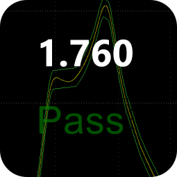
Click OK, and then press Run. You should be greeted with a screen indicating pass/fail if every measured point falls inside the mask:

The mask file is just a text file. We can edit it directly to skip or change certain regions. For example, the notch at about 3.3 kHz is very deep. If you go into the mask file, you can see the first column is the frequency, the second column is the lower mask Y value, and the third column is the upper mask Y value. You can change this as as needed, or you can make a region to be "don't care" by setting the beginning and ending frequency of a region to be NaN (not a number).
When this is done for the frequencies between 3 and 3.4 kHz, the mask file is changed as follows. In a text editor, all the rows from 3 to 3.4 kHz were selected and deleted and then the NaN values were inserted. Save the text file, then go back into the FR context menu and re-load the mask file you just changed.

The resulting display now shows a gap in the mask from 3 to 3.4 kHz. The measured signal could be anything in that region and still pass. Or we could simply create a larger and more forgiving box.

Summary
The next step will be to roll the notion of masks into Tractor in the next week or so. Tests will be added to Tractor to allow you specify a sweep, and then perform actions on that measured data. One of those actions will be to measure against a mask.
What was shown above was a somewhat contrived experiment using low-cost laser-cut fixturing to make a fairly repeatable test stand for production testing. This may or my not have applicability to what you need to measure. The repeatability was good at roughly +/- 1 dB. A MEMS mic was used to keep the space requirements modest and predictability high given the robust nature of MEMS microphones and their highly accurate fabrication process. And finally, the QA401 software was used to build a statistical model of the measurements, establish 4 sigma limits, and generate a mask from the initial measurements. The mask generated was roughly +/- 1.5 dB in areas away from resonant peaks. A more rigorous treatment would collect the curves of 10 to 20 units, generate a mask from that collection, and then edit the associated mask file to ignore the wild response at frequencies beyond 10 kHz or so that come from not using a chamber.
Or, you can make the measurements in a chamber and enjoy the improved consistency. Considering a lot of factory testing today is looking simply at dBSPL at a single tone and is measured using an operator with a SPL meter, the improved test coverage and accuracy should be viewed as a good next step, even if not done within a chamber.
Like what you just read? Join our mailing list at the bottom of the page.