
Quantifying Fuzz
In release 1.709 for the QA401, the ability to graph distortion versus level for a given frequency was added. This is achieved using the new Test Plug-in “Gain and Distortion versus Amplitude”. This can be accessed from the main menu using the Test Plugins->Gain and Distortion selection. Most audio amplifier designers won’t really benefit from this plug-in, as its purpose is to help those designing circuits that intentionally add distortion to a signal: guitar pedals and effect processors. For these devices, it’s often very helpful to see the type of distortion that’s being introduced as well as how it’s being introduced.
We’ll take a look at three distortion units. The first is a Line 6 Spider III 15W amplifier. This is a low-cost practice amp that does a reasonable job of giving the player a fairly broad palette of tones and effects for a decent price. The second is a very low-cost overdrive pedal we looked at previously: the Koko Overdrive. The final unit is a Behringer V-Amp Pro multi-effects in a rackmount form actor.
Plugin in Loopback
Before we start on the effects, let’s first take a look at the new plug-in in loopback mode on the QA401. That is, we take the output of the QA401 and connect it directly to the input. First, we specify the parameters of the sweep. We’d like to sweep a 1 KHz tone from -120 dBV to 5 dBV.

A video of the process shows how quickly the graph is generated. Note that smaller FFT sizes will run even faster, but with less accuracy. And longer FFT sizes will run more slowly, but with more accuracy. You can select the FFT size depending on what you are after. In general, with noisier equipment such as pedals and guitar amps, the smaller FFT sizes (such as the 8K used here) are fine.
The output from the video above is the following graph, where you have input level in dBV on the X axis, Gain in dB shown on the left Y axis, and THD in dB shown on the right Y axis.
A shaded region was added to show where the magnitude of the gain linearity exceeded 0.5 dB. In other words, you can see that at very small output levels (-110 dBV is 3.16 uVrms) you will actually get a little bit more from the QA401 that you have dialed in. At the most extreme, if you specify -120 dBV (1uVrms) you will actually get -118.5 dBV (1.2uVrms).
The key point is that this plot makes it very easy to see where your equipment is exhibiting gain linearity. A flat horizontal blue line is what you want to see if your aim is fidelity.

In the same plot below, the shaded region highlights the distortion measurement. The red line is the overall distortion, and the green and purple lines are the 2H and 3H harmonics. This makes it easy to see if the distortion you are seeing is primarily even or odd in nature. The fact that there’s a gap between the 2H and 3H lines and the red line indicates that something else is driving the overall distortion measurement. It could be a 5H harmonic, which wouldn’t be shown, or it could be the system noise floor. Most always the gap will mean that you are noise-limited and in the noise floor region. In the region highlighted in the plot below, the THD is limited by noise. If you are using a small FFT and want to be seeing harmonics instead of noise, then increasing the size of the FFT will push the noise down.

In the last shaded region below, we are no longer noise limited. You can see this because the 2H and 3H components, when added, would equal the red THD line. In other words, the distortion is rising at this point and the distortion is no longer limited by noise. This is real harmonic distortion overwhelmingly comprised of 2H and 3H products.

Koko Overdrive
Next, let’s take a look at the same plugin used on a guitar pedal: The Koko overdrive. For the pedal test, we’ll use 220 Hz as the stimulus. A low E on a guitar is about 82 Hz, so this puts us a about 1.5 octaves above the low E. Tthe high E string on the guitar is about 330 Hz. An octave above that would be 660 Hz. And an octave above that—which would be the highest note you could reasonably play on an electric guitar with bending, would be 1.32 KHz. Thus, the fundamental notes of a guitar range from about 82 Hz to 1.3 KHz.

In the plot above, we see the pedal is largely linear in its gain out to about -40 dBV input. At that point, the input starts getting compressed heavily.
We can also see the pedal is giving just a bit of gain--just shy of 2 dB. The purpose of an overdrive, versus a distortion pedal or fuzz pedal, is to make the input into your amp just a bit "hotter" and with a hint of distortion. This pedal is doing just that.
What is important to notice here is the distortion is dominated by 3H—the purple curve hugs the red THD trace. Odd distortion (3H, 5H, etc) is generally heard as sounding a bit warmer, “rounder”, and pleasing. The spectrum at -20 dBV appears as below, and you can see a single cycle of the time-domain waveform inset in the graph.

Line 6 Spider III 15W
Next, we repeat the experiment using a Line 6 Spider III 15W amplifier. This is a solid-state amp, relying on an ST Micro TDA2030 power amp stage and some digital processing to approximate the distortion and EQ. The power amp IC is rated at 18W, while the guitar amp is rated at 15W. For the settings below, all knobs were set to mid point unless noted. Drive was max, and the headphone output was used with the Master setting at about 9 o’clock.

The shaded region of the Line 6 reflects a messy noise floor. The signal in this area is far below countless spurious products in the output. Beyond about -60 dBV input, peak gain is about 35 dB, and the gain compression occurs after -45 dBV. Remember, the overdrive pedal was just a few dB of gain. This amp is 35 dB.
The spectrum and time domain are both shown below for the -20 dBV input level:

Behringer V-Amp Pro
Lastly, we look at a Behringer V-Amp Pro. This is a rack-mounted multi-effects processor.
First plot is the setting American Blues, with all knobs mid and master straight up. This unit employs a noise gate (shaded region). What is interesting here is the distortion is primarily 2H until you get to about -30 dBV, and then moves quickly to 3H. So when plucking more quietly, the distortion is fairly subtle: it’s just a some 2H added in around about 30 dB below the fundamental. But as you pluck harder, the 3H comes on hard at just a few dB below the fundamental. The V-Amp does have a very pleasing blues patch. The transition from 2H to 3H distortion ads a layer of tonal expression otherwise not present in a pure 3H distortion circuit.

Looking at the spectrum for a -20 dBV input, we see what the graph above conveys clearly. The inset shows the time domain, and it’s clear there’s some a fair bit of asymmetry too.

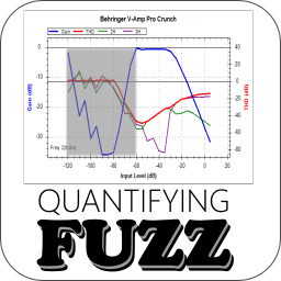
Finally, we look at the V-Amp with the Crunch setting:

Note the mechanism used to generate the distortion is exactly the same: We see it begins with heavy 2H, and the shifts to heavy 3H. We also get just over 10 dB more gain.
If we do a sweep of the frequency response for both settings (using the Frequency Response plugin), and opt for overlaying of the data, we get the following:

For the blues setting, the low end was scooped by about 15 dB. For the Crunch setting some mids were scooped. Both relied on plenty of gain up around 2-3 KHz.
What this means
In deciding your test strategy, you can look at the various regions of operation during development to decide what measurements you’d need to make during testing. There’s not a really a reason to replicate the full graph during test. Instead, you can make instead several discrete measurements at the indicated points.

Point 1 would be a measurement made to ensure the pedal’s noise floor is functioning correctly. That is, you’d first make a measurement with no signal present and capture the noise floor. Then, you’d make a measurement with a signal at a level perhaps 10 dB out of the noise floor and verify the amplitude is correct. If your noise floor or dynamic range is degraded, this is an easy way to detect it.
Point 2 would be a measurement made to verify the linearity is holding just before the compression knee occurs.
Point 3 would be a measurement made to ensure the knee isn’t too steep or too shallow. This could be due to a distortion diode installed backwards or missing.
Point 4 would be a measurement made to ensure the max signal handling capability of the pedals is functioning as designed. This is a very quick test to know your supply rails are functioning correctly. You can often deduce the correctness of the supply rails (without having to measure the supply rails) by applying an abnormally large signal to the input. If the supplies rails aren’t where they should be, then the THD will rapidly climb as the opamp runs out of headroom.
Each of these measurements is very quick to automate and make on Tractor. The four measurements above would take just seconds in a production environment.
Summary
If you are designing circuits aimed at inducing distortion, this new plug-in can be very helpful for seeing some key transition points in your circuit’s operation. It can also help you understand where you want to test circuit operation in the manufacturing process.