

TI TPA3255 EVM
Later this week 1.726 will release, with a lot of changes to plug-ins and graphing of stepped tests. The aim over the last month has been to dramatically improve work flow and reduce or even eliminate the need to go into to Excel for graphing more complex scenarios. The scenarios to consider are along the lines of "I'd like to see a graph of my amp's IMD performance on the left channel for both 4 and 8 ohms, and I'd like to compare that to some series I previously measured from an older board at both 4 and 8 ohms...all on the same graph."
Normally, a graph like that gets a bit sticky to make. You can export everything and load it up in Excel, but that takes time. And Excel isn't so useful when you want to create a graph of a fixed size (say, 800x480 pixels). You can of course screen capture the plot Excel it and re-size it in another program, but the aim here is to make it wickedly fast to capture and present fairly complex data without a lot of intermediate steps.
With the new release, the above scenario would be accomplished by measuring IMD performance at 8 ohms to initially create the graph, and then running it again at 4 ohms and directing that output of that sweep to the graph you just made (instead of a new one), and then importing the old data into the graph with the two traces. And along the way, you can interactively play with scaling, axis names, colors, import/export, etc.
The purpose of this blog post is to show how to quickly evaluate an amplifier using many of the new features and plug-ins in the 1.726 release.
TI's TPA3225 EVM
About 18 months ago we looked at a generic TPA3255 board that was a reasonable performer. In that evaluation, the tests made were mostly single-point snapshots. And when showing the frequency response, the data was plotted in Excel. What you should takeaway in the evaluation below is how much of the testing today has become completely automated, the breadth of the tests that can be performed, and the speed. At the end of the day, the goal is to help you understand your products quickly.
Let's get started...
For the tests below, the connection diagram is shown below. The QA450 doesn't need to be used here: you could manually connect a load as required for the tests. We're using the QA450 in manual mode in these tests. In manual mode, you change loads (4 or 8 ohms) by pressing on-screen buttons. The QA450 also supports automated control via REST.

The supply used for all of the tests below is a 48V/10A ACDC brick, with the trimpot dialed up to 51V. This limits some of the testing because it cannot supply enough current for drive both the left and right channels to maximum power. For most plots below, the data was collected on the left channel only.
The noise of the amp at 51V was verified with a lab supply to ensure the brick wasn't degrading the amp performance with its own noise. It was not. TI's EVM doesn't care whether you are using a lab supply or an economical fixed ACDC supply.
Mutlitone
A good first test when first trying to understand an amplifier is a multi-tone test, because it provides a quick way to look at the gain, gain balance, the flatness of the spectrum and the cross-talk all at once.
The total RMS power from 20 to 20 KHz using a multi-tone stimulus is about 17.3W into 8 ohms in the plot below. From the text display at the bottom of the graph we can see the amp has a gain of roughly 27.5 dB, exceptional (0.01 dB) matching between the channels, about -75 dB of cross-talk, and just a bit of roll-off (about 0.4 dB) up near 20 KHz. Generally, we might state the gain of the amp is 27.5 dB +0/-0.4 dB. And no worrisome spurious products are observed.
Here the Multitone QA401 output level is -6 dBV (total RMS in 20 to 20 KHz). For inputs lower than -6 dBV into the TPA3255, the spectrum appears very similar.

Nudging the QA401 multitone output up 1 dB to -5 dBV input shows a picket fence of products suddenly appearing--growing about 30 dB in the process (see plot below). The CLIP_OTWZ LED also flickers on the EVM. This LED by itself suggests that the junction temperature is higher than 125C according to Table 2 in the EVM. But the total RMS of all the tones is 22.4 DBV which is about 22W.
What is going on? How can a 300W amp be putting out just 22W and increasing the input by 1 dB cause its performance to collapse?

The answer is the the crest factor: While the RMS of the 12 tones is 22.4 dBV = 13.18 Vrms, the momentary peak of the signal can result in a short excursion on a single terminal of +/-25V across the load as verified with a scope. This means that's a total of 50V across the speaker--and at that point the amp has run out of supply rail and/or is current limiting and/or is also fighting on-die thermal limits due to the instantaneous dissipations encountered. In short, multi-tone is a great tool, but make sure you understand that is incredibly demanding on the equipment and it's easy to push things too hard (Some quick math: A single sine has a crest factor of 20 * Log10(1/0.707) = 3 dB. Worst case, the 12 tones in the multi-tone test sequence could potentially peak at 36 dB above the RMS. Be careful!)
Dialing the output back to -7 dBV and switching to a 4 ohm load we see the following:

This time we see the Peak- is reported as -1.75 dB. That is the minimum amplitude of one tone is about 1.75 dB below that of the mid-band tone. And visually we can see that is happening at the 20 KHz frequency.
So, the act of changing from an 8 to a 4 ohm load has resulted in the frequency response of the amp dropping at 20 KHz by about 1.4 dB. And this shouldn't be a surprise: Class D amps require the output filter be designed for a specific load. If you change the load, the output response will change.
OK, thus far we have some import information: Nominal gain is around 27.5 dB and there's a bit of droop at the higher end with lower impedances.
Frequency Response
Multitone looks across the band with a dozen frequencies. But let's take a more detailed look at the frequency response at 4 and 8 ohms. For this, we'll sweep from 20 to 20 KHz at -18 dBV into the TPA3255. With an 8 ohm load this will give about 1W of output. For this test, the sampling rate on the QA401 was set to 192 Ksps and Flat Top windowing was used.

After running the sweep, we're presented with the following graph. This is a new window introduced in the last month or so. Notice the ability on the left side of the dialog to customize trace colors, thickness, names, etc. For now, we'll do nothing and just take the graph as is.

Next, we switch the load to "4 ohms" on the QA450 programmable load:

And then we run the exact same sweep again, just as we did above. This time, after the sweep completes, we're presented with a new option:

The Graph Selection dialog box is saying "I notice you have at least one graph window already open. Do you want to add this new sweep to an existing graph OR do you want add it to a new graph?"
The "QA401 Graph 112" matches the title bar in the first graph we generated. The "112" is just a random 3 digit number to disambiguate the different graph windows.
Let's opt to add it to the existing window. And now we're greeted with:
The graph above needs tweaking. The trace colors are the same, the title is ambiguous and trace names aren't helpful. Let's use the features of the graph tool to fix this (changing colors, adding notes, changing titles) and then copy 800x480 sized bitmap to the clipboard for pasting into this post:

From the plot above, we can readily see the response at 20 KHz is about 1.6 dB down with a 4 ohm load versus an 8 ohm load. The gain of the amp is also reduced a bit due to the amp output impedance, which we'll look at in more detail below.
But in short, this is a big improvement over previous versions of the application. No import/export, finding traces in directories, remembering the names, etc.
In the section below looking at output impedance we discuss this load sensitivity a bit more.
Next, we'll move on to look at amp distortion.
THD+N
Like the frequency response sweep, capturing a THD+N versus power takes just a few seconds to run. The setup for this test is shown below, with some new options highlighted.

The first option is that the QA401 application can manage the attenuator automatically for you. This is helpful because at lower levels of power out, having the attenuator off will lower the noise floor. If you elect to have the plug-in manage the attenuator, then the measurement will always start with the attenuator active. From there, the plug-in will decide when it makes sense to enable the attenuator. Generally, this will occur at around -20 to -10 dBFS, depending on whether you are measuring THD or THD+N.
Switching the attenuator automatically has a downside in that it introduces a bump in your output display, which usually will need some explanation if you are presenting the data to others. So, if your application isn't showing a difference at lower levels with attenuator on and off, then leave the attenuator on and take the glitch-free trace. The TPA3255 is an exceptional performer, and for that reason the data presented below lets the plug-in manage the attenuator.
The second highlighted checkbox is the ability to enable an early abort of the test sequence. This is helpful if you don't know the limits of the amp, but you know you want to stop as soon as the THD (or THD+N) exceeds a certain threshold. In the example above, we see the Abort Minimum Power Level is 10W, and the Abort Maximum THD is -85 dB. With these settings, if enabled, the plug-in would automatically stop at any measurement where the measured power was greater than 10W AND the THD had exceeded -85 dB.
The resulting output from the THD+N sweep is below. In the above settings, note that we elected to have the plug-in manage the attenuator. You can see where the plug-in engaged the attenuator. Also we now have THD+N displayed in both dB and as a %.
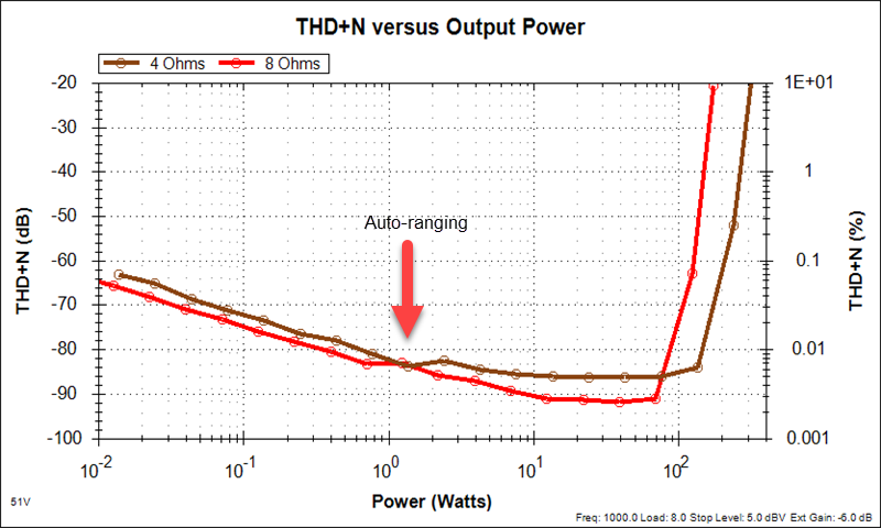
How does this compare with TI's sweep of the part? That graph is below. TI has a lot of additional filtering that was used on their measurement, including an AES17 and AUX-0025. They also ran the test at 75C. The distance between power steps looks very small (1 dB or less versus the 2.5 dB steps taken above).
But in any case, the two plots compare quite favorably, and it took just a few minutes to setup, run and prepare the graph.

IMD
A sweep of IMD is important on Class D amps as it's difficult to measure linearity at higher frequencies using a conventional THD techniques because the world beyond 50 KHz in Class D amps is usually fairly harsh. Below is the setup for the IMD measurement. That this time we are enabling early termination: If the power level exceeds 1W AND the IMD exceeds -60 dB, then the sequence will terminate early.

There isn't an option for the type of IMD measurement right now in the above configuration (ie, SMPTE or ITU), but there will be at some point. The test above will measure the level at 1 KHz while applying a 19 KHz and 20 KHz tone at equal levels (commonly known as the ITU-R or CCIF/ITU). If you specify an output level of 0 dBV, then the level of each tone will be -3 dB, and the combined RMS of the two non-coherent tones will be 0 dBV. The response at 1 KHz is referenced to the combined RMS of the two tones. In the future will be the ability to specify the max order of distortion. Currently, a single second-order product is considered (F1 = 19K, F2 = 20K, and ABS(1* 19K - 1* 20K) = 1 KHz.).
A previous post talks more about IMD measurements (including background) on the QA400.
The resulting plot of the IMD measurement is as follows. TI doesn't publish IMD figures on the TPA3255.

A plot of about 10W into 8 ohms shows the following activity. We can see the total RMS of the 19 and 20 KHz tones are 19 dBV, and the amplitude of the resulting 1 KHz tone product is about -84 dBV, resulting in measurement of about -103 dB.

Output Impedance
Measuring output impedance of an amplifier is done by taking measurements of the output across two loads, usually an open and a typical speaker load, or in this case, a 4 ohm (instead of an open) and 8 ohm load. And then through some algebra we can compute the output impedance of the amplifier. The setup screen for this plug-in is below. We'll first sweep at 8 ohms, and then sweep at 4 ohms. We'll also do the left and right channel together:

When the test starts, we're instructed to first connect the 8 ohm load. With the QA450, we make sure the 8 ohm button is pressed.

That sweep will take a few seconds, and the we see the second prompt. There we connect the 4 ohm load:

Upon completion of the second sweep, we get the following graph of output impedance:

At 1 KHz with a 4 ohm load, this is a damping factor of roughly 30. At 20 KHz, the output impedance is nearly 2 ohms. This is overwhelmingly coming from the output LC filter. The output L is 15 uH, which has an impedance of 1.8 ohms at 20 KHz.
This highlights a common complaint with class D. Historically, class D amps have had three big problems: Poor PSRR, marginal to poor output impedance (especially at higher frequencies), and poor tolerance to load changes (as we saw above in the frequency response of 4 versus 8 ohms).
TI has addressed the first problem of PSRR by closing the loop on the TPA3255. But the second and third problems are due to the output LC. And TI only closed the loop prior to the LC in the TPA3255. In the future, look towards class D chipsets than can close the loop using feedback taken post-LC. The math and processing to do so must be very difficult. But you can bet the big class D chipset companies are working hard to solve this.
Noise
A noise measurement was made with the inputs shorted and with A-Weighting enabled. TI's spec indicates a typical 85 uVrms noise (20 to 20 KHz), and what was measured below was 95 uVrms. This measurement was into 4 ohms.

Gain Linearity
The gain of an amplifier should be linear across it's operating region. That is, if the amp gain varies based on the incoming signal level, it can result in strange amplitude modulations.
The graph below is the setup for the gain linearity test. The set up indicates we'll sweep the QA401 output from -120 to +5 dBV, in 5 dBV steps, and measure the gain at each point. What we'd like to see is a single horizontal line.

The plot from the test is shown below. There are 3 regions to note: The first is left side of the graph below -110 dBV or so input level. Here we can see that if a very small signal is input to the amp, then the gain is around 28.5 dB.
And on the far right side, with very high input levels around +5 dBV, the gain drops to about 26.5 dBV.

What we see above on the far left side of the graph and on the far right are to be expected. The key is the steller performance in the middle region from -110 dBV to just over a few dBV of input.
On the left side, the deviation can be explained by noise. The signal is so small that its difficult to separate the noise from the signal. But it doesn't matter, because we're not able to hear the signal at this level either.
And on the right side, the deviation can be explained by amplifier compression. But at this level, the output is so large (200 to 300W) it just doesn't matter. In summary, the gain linearity of this part is very good.
A side note on the QA450 and Power Handling
In many of the above tests, that the power into the QA450 was exceeding 300W in some cases (the manual has more analysis on this). The QA450 cannot handle these levels of power for very long. But if you are doing swept tests with smaller FFT sizes, it can handle them for long enough periods to make the measurement.
And this is an important point to make again: The QA450 isn't designed for sinking hundreds of watts for several minutes. It's designed for making very fast measurements at several hundred watts under automated control.
Conclusion
Overall, the new plug-ins should really help expedite your work flow and minimize the amount of time you need to spend in external graphing programs for most daily work. If there's a measurement you routinely make that you think needs to be streamlined, drop us an email.
If you liked the post you just read, please consider signing up for our mailing list at the bottom of the page.